If you are here, you are already introduced to the concept of logistic regression and probably have had your hands dirty working on different datasets. The scikitlearn’s LogisticRegression is by far the best tool to use for any logistic regression task, but it is a good exercise to fiddle around and write your logistic regression algorithm and see how your algorithm fares. It always helps a great deal to write algorithms from scratch, provides you with details that you otherwise have missed, It consolidates your knowledge regarding the topic. It will be helpful if you have a prior understanding of matrix algebra and Numpy. In this article, we will only be dealing with Numpy arrays. Well, let’s get started,
This article was published as a part of the Data Science Blogathon.
Table of contents
Import libraries for Logistic Regression
First thing first. We will first import the necessary libraries and datasets. In this article, we will only be using Numpy arrays.
import numpy as np
from numpy import log,dot,e,shape
import matplotlib.pyplot as plt
import dataset
For this article, we will be using sklearn’s make_classification dataset with four features:
from sklearn.datasets import make_classification
X,y = make_classification(n_features = 4,n_classes=2)
from sklearn.model_selection import train_test_split
X_tr,X_te,y_tr,y_te = train_test_split(X,y,test_size=0.1)

print(X_tr.shape, X_te.shape)
Standardization
Standardization is the process of scaling data around the mean with a unit standard deviation. That means we are effectively making the mean of the attribute zero with the resulting distribution having a standard deviation equal to zero. Some algorithms are vulnerable to features with different scales. Especially if we are using gradient descent for optimization, then the model will have a hard time giving accurate results; for example, if a dataset has two features, age and salary, then the salary feature with its higher range will most likely dominate the outcome. So, it is a good practice to standardize data before feeding it to the algorithm. Highly recommended to go through this article to understand standardization clearly. Mathematically it is given as
This is often necessary when attributes are from different scales.
def standardize(X_tr):
    for i in range(shape(X_tr)[1]):
        X_tr[:,i] = (X_tr[:,i] - np.mean(X_tr[:,i]))/np.std(X_tr[:,i])
Initializing Parameters
The data sets are always multidimensional. We will need to use matrices for any kind of calculation. So, for input, we have two matrices to deal with. The first one is for feature vectors, and the second is for parameters or weights. Our first matrix is of the mxn dimension, where m is the number of observations while n is the dimension of observations. And the second one is of nx1 dimension. Here, we will add a bias column of ones to our feature vectors matrix and a corresponding parameter term to the weight vector. Bias is important to make the model more flexible.
    def initialize(self,X):
        weights = np.zeros((shape(X)[1]+1,1))
        X = np.c_[np.ones((shape(X)[0],1)),X]
        return weights,X
Note: In the code above, although we have initialized the weight vector to be a vector of zeros, you could opt for any other value as well.
Sigmoid Function
In a linear regression model, the hypothesis function is a linear combination of parameters given as y = ax+b for a simple single parameter data. This allows us to predict continuous values effectively, but in logistic regression, the response variables are binomial, either ‘yes’ or ‘no’. So, it makes less sense to use the linear function to predict anything except the values between 0 and 1. And the most effective function to limit the results of a linear equation to [0,1] is the sigmoid or logistic function.
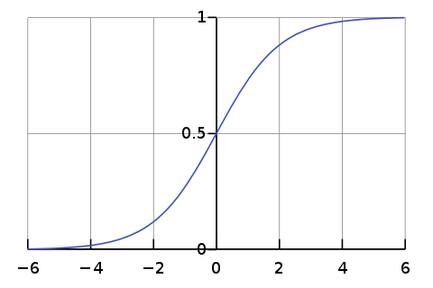
As you can see, the sigmoid function intersects the y-axis at 0.5. In most cases, we use this point as a threshold for classification. Any value above it will be classified as 1, while any value below is 0. This is not a rule of thumb. We can also use different values instead of 0.5, depending on the requirements. The sigmoid function:
We plug the linear equation in place of x.
python code:
    def sigmoid(self,z):
        sig = 1/(1+e**(-z))
        return sig
In the above expression, z is the dot product of the mxn matrix containing observations and nx1 matrix of weights.
Cost Function
Cost function or loss function is that function that describes how much the calculated value deviates from the actual value. Linear regression employs the least squared error as the cost function. But the least squared error function for logistic regression is non-convex. While performing gradient descent chances that we get stuck in a local minimum is more. So instead, we use log loss as the cost function.
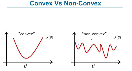
Image source: www.fromthegenesis.com/artificial-neural-network-part-7/
The formula gives the cost function for the logistic regression.
Where hx = is the sigmoid function we used earlier.
python code:
        def cost(theta):
            z = dot(X,theta)
            cost0 = y.T.dot(log(self.sigmoid(z)))
            cost1 = (1-y).T.dot(log(1-self.sigmoid(z)))
            cost = -((cost1 + cost0))/len(y)
            return cost
Gradient Descent
The next step is gradient descent. Gradient descent is an optimization algorithm that is responsible for the learning of best-fitting parameters. So what are the gradients? The gradients are the vector of the 1st order derivative of the cost function. These are the direction of the steepest ascent or maximum of a function. For gradient descent, we move in the opposite direction of the gradients. We will be updating the weights in every iteration until the convergence. The pseudocode for Gradient descent looks something like this.
Here, the alpha is the step size responsible for how quick it converges to the global minimum. If the step size is too small, it will converge slowly, but if it is too large, it may overshoot the minimum while descending.
By differentiating the cost function, we get the gradient descent expression
or,
This is the vectorised form of the gradient descent expression, which we will be using in our code.
    def fit(self,X,y,alpha=0.001,iter=100):
        params,X = self.initialize(X)
        cost_list = np.zeros(iter,)
        for i in range(iter):
            params = params - alpha * dot(X.T, self.sigmoid(dot(X,params)) - np.reshape(y,(len(y),1)))
            cost_list[i] = cost(params)
        self.params = params
        return cost_list
Prediction
Everything that we have done far is for this step. We trained the model on a training dataset, and now We will use the learned parameters to predict the unseen data.
    def predict(self,X):
        z = dot(self.initialize(X)[1],self.weights)
        lis = []
        for i in self.sigmoid(z):
            if i>0.5:
                lis.append(1)
            else:
                lis.append(0)
        return lis
F1-Score
Now that we are done with the prediction, we will move on to the F1-score section, where we will measure how good our model predicts for unseen data. The F1_score is a robust metric for evaluating the performances of classification models, and mathematically F1-score is the harmonic mean of precision and recall.
precision = Precision is the number of true positives over the sum of true positives and false positives
precision = TP/(TP+FP)
recall = Recall is the number of true positives over the sum of true positives and false negatives.
recall = TP/(TP+FN)
def f1_score(y,y_hat):
    tp,tn,fp,fn = 0,0,0,0
    for i in range(len(y)):
        if y[i] == 1 and y_hat[i] == 1:
            tp += 1
        elif y[i] == 1 and y_hat[i] == 0:
            fn += 1
        elif y[i] == 0 and y_hat[i] == 1:
            fp += 1
        elif y[i] == 0 and y_hat[i] == 0:
            tn += 1
    precision = tp/(tp+fp)
    recall = tp/(tp+fn)
    f1_score = 2*precision*recall/(precision+recall)
    return f1_score
Putting Everything Together: Logistic Regression
Now that we are done with every part, we will put everything together in a single class.
import numpy as np
from numpy import log,dot,exp,shape
import matplotlib.pyplot as plt
from sklearn.datasets import make_classification
X,y = make_classification(n_featues=4)
from sklearn.model_selection import train_test_split
X_tr,X_te,y_tr,y_te = train_test_split(X,y,test_size=0.1
def standardize(X_tr):
    for i in range(shape(X_tr)[1]):
        X_tr[:,i] = (X_tr[:,i] - np.mean(X_tr[:,i]))/np.std(X_tr[:,i])
def F1_score(y,y_hat):
    tp,tn,fp,fn = 0,0,0,0
    for i in range(len(y)):
        if y[i] == 1 and y_hat[i] == 1:
            tp += 1
        elif y[i] == 1 and y_hat[i] == 0:
            fn += 1
        elif y[i] == 0 and y_hat[i] == 1:
            fp += 1
        elif y[i] == 0 and y_hat[i] == 0:
            tn += 1
    precision = tp/(tp+fp)
    recall = tp/(tp+fn)
    f1_score = 2*precision*recall/(precision+recall)
    return f1_score
class LogidticRegression:
    def sigmoid(self,z):
        sig = 1/(1+exp(-z))
        return sig
    def initialize(self,X):
        weights = np.zeros((shape(X)[1]+1,1))
        X = np.c_[np.ones((shape(X)[0],1)),X]
        return weights,X
    def fit(self,X,y,alpha=0.001,iter=400):
        weights,X = self.initialize(X)
        def cost(theta):
            z = dot(X,theta)
            cost0 = y.T.dot(log(self.sigmoid(z)))
            cost1 = (1-y).T.dot(log(1-self.sigmoid(z)))
            cost = -((cost1 + cost0))/len(y)
            return cost
        cost_list = np.zeros(iter,)
        for i in range(iter):
            weights = weights - alpha*dot(X.T,self.sigmoid(dot(X,weights))-np.reshape(y,(len(y),1)))
            cost_list[i] = cost(weights)
        self.weights = weights
        return cost_list
    def predict(self,X):
        z = dot(self.initialize(X)[1],self.weights)
        lis = []
        for i in self.sigmoid(z):
            if i>0.5:
                lis.append(1)
            else:
                lis.append(0)
        return lis
standardize(X_tr)
standardize(X_te)
obj1 = LogidticRegression()
model= obj1.fit(X_tr,y_tr)
y_pred = obj1.predict(X_te)
y_train = obj1.predict(X_tr)
#Let's see the f1-score for training and testing data
f1_score_tr = F1_score(y_tr,y_train)
f1_score_te = F1_score(y_te,y_pred)
print(f1_score_tr)
print(f1_score_te)
output:0.9777777777777777
0.9090909090909091
Now. let’s see if our cost function is descending or not
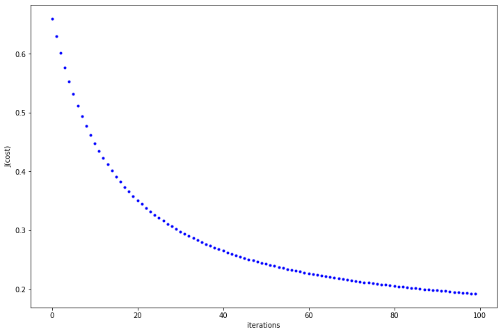
In the above plot, we can see that the cost function decreases with every iteration and almost gets flattened as we move towards 100. You can fiddle around with hyper-parameters and see the behaviour of cost function.
Now, let’s see how our logistic regression fares in comparison to sklearn’s logistic regression.
from sklearn.linear_model import LogisticRegression
from sklearn.metrics import f1_score
model = LogisticRegression().fit(X_tr,y_tr)
y_pred = model.predict(X_te)
print(f1_score(y_te,y_pred))
output: 0.9090909090909091
Great!
Logistic Regression EndNote
This article went through different parts of logistic regression and saw how we could implement it through raw python code. But if you are working on some real project, it’s better to opt for Scikitlearn rather than writing it from scratch as it is quite robust to minor inconsistencies and less time-consuming.
Happy coding!
The media shown in this article is not owned by Analytics Vidhya and are used at the Author’s discretion.
Meet your author Sunil kumar Dash, a developer and a writer. Has diverse interests in tech, pop culture, wellness, philosophy and Anime. Exploring underrated music is his hobby. And loves to doom scroll Twitter when bored.


Line 7 you have to close the bracket :)