Optimal Resource Allocation using Python

This article was published as a part of the Data Science Blogathon.

Objective

“True optimization is the revolutionary contribution of modern research to decision processes” – George Dantzig.

This article discusses solving a resource allocation problem using linear programming in Python. We will find an optimal value for a linear equation with different linear constraints. We can solve linear programming using the PuLP library, and other Python libraries that can perform similar tasks are SciPy, Pyomo, CVXOPT. Let’s discuss associated concepts and problem statements in detail.

Appreciating PuLP

PuLP is an LP modeler written in Python. It can use solvers like CBC, GLPK, CPLEX, MOSEK, etc., to name a few, solve linear problems. The default solver is CBC. It requires Python 2.7 or Python >= 3.4. Some commonly used classes used in PuLP are –

1. LpProblem – used for defining a problem

2. LpVariable – used to create new variables

3. LpConstraint – used to create constraints

4. Ipsum – to create a linear expression of the form a1*x1 + a2*x2

5. Value – used to get the value of the variable or expression

We can refer to this document for further reading

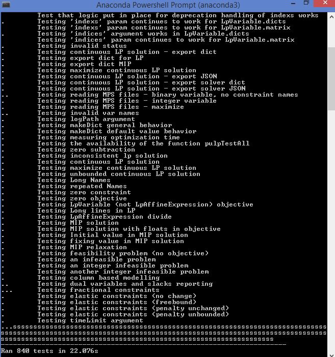
We can test pulp after importing as

import pulp
pulp.pulpTestAll()

The result can be seen as

Pulp Models

PuLP models can be saved, exported, and reused in another machine or other times. There are two ways to export a model –

1. MDS format

We can use the following commands to store the model

model.writeMPS("model.mps")

We can use the following control to retrieve the model

var, model = LpProblem.fromMPS("model.mps")

We will print both variables to check

print(var)
print(model)

2. Dictionary format

We can use
the following commands to store the model in a dictionary

M1 = model.to_dict()

We can use the
following to retrieve the model

var, model = LpProblem.from_dict(M1)

We will print both to check the output

print(var)
print(model)

Linear Programming

A linear program is a mathematical program that satisfies three conditions –

1. Decision variables must be real

2. The objective function must be linear

3. The constraint equation must be linear

Linear programming aims to maximize or minimize a numerical value, and it is considered one of many techniques used to find optimal resource utilization. The different aspects of linear programming are decision variables, constraints, data, and objective function, and we will discuss these in detail in the next section. Linear optimization applications are in the manufacturing industry, transportation industry, engineering, energy industry, etc.

Steps of optimization are –

1. Setting a problem statement – For example, we need to allocate resources optimally across three locations for two works

2. Formulating equation – we need to identify decision variables to form an objective function. For example, considering the cost of the resources, the number of works, and locations, objective function will be arrived at.

3. Solving the equation – we can use any one of the solvers mentioned above to arrive at optimal values

4. Post analysis – Once arrived at the optimal solution, we need to fit it along with the business objective to check if all business constraints are also satisfied

5. Presenting the solution – The optimal solution should make sense and be presented for stakeholders to arrive at decisions

Default Solver

PuLP’s default solver is CBC (Coin-or branch and cut). It is an open-source mixed integer programming solver. It is written in C++, and it can be used with other coin projects for more functionality like Clp, Cgl, CoinUtils.

The puLP can list solvers using the following commands –

import pulp as plp
plp.listSolvers()

We
can get desired solvers using

getSolver()

Resource allocation Problem

The resource allocation problem is an optimization problem. It seeks to find the optimal allocation of resources across locations and tasks. Each resource has an associated cost, and the number of resources is fixed. In our code, we have treated the number of resources for each work to be an integer. Resource allocation optimization can be applied in production planning, queueing, load distribution, etc. The aim is to minimize the total cost and maximize production.

Terminology

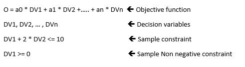
1. Objective function: It is a linear equation which we try to maximize or minimize

2. Decision variables: These are variables used in the equation

3. Constraints: These are restrictions or limitations on the decision variables

4. Non-negative rules: Decision
variables values should be positive

Illustrating the four terms through the equation below

Problem Statement

There are three locations – location1, location2, location3. There are two works – work1, work2. Each location has resources, each position requires resources, and each resource has a cost associated with it. We have to optimally allocate work in each place to minimize overall resource costs.

Implementation

Importing Libraries

We will use Pandas, NumPy, and PuLP libraries. Details for the PuLP library are explained in the sections above.

import pandas as pd
import pulp as plp
import numpy as np

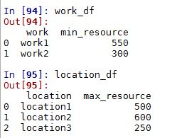
Creating the input variables

We will create two data frames – for location and work resource constraint and one array for the cost of resources. These three variable values are sample inputs, and we can replace them with actual data for actual results.

location_df  = pd.DataFrame({'location': ['location1', 'location2', 'location3'],
                             'max_resource':[500, 600, 250]
                             })
work_df  = pd.DataFrame({'work': ['work1', 'work2'],
                             'min_resource':[550, 300]
                             })
resource_cost = np.array([[150,200], [220,310], [210,440]])

Defining model

Since it is a minimization problem, we will use LpMinimize

model = plp.LpProblem("Resource_allocation_prob", plp.LpMinimize)

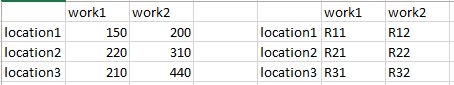
Creating objective function

We will create an objective function considering the resource cost array defined. Here 150, 200, and so on are the cost of resources R11, R12, etc. The below picture shows the number of variables created in the objective function. R11, R12, R21, R22, R31, R32 are the decision variables.

no_of_location = location_df.shape[0]
no_of_work = work_df.shape[0]
x_vars_list = []
for l in range(1,no_of_location+1):
    for w in range(1,no_of_work+1):
        temp = str(l)+str(w)
        x_vars_list.append(temp)
x_vars = plp.LpVariable.matrix("R", x_vars_list, cat = "Integer", lowBound = 0)
final_allocation = np.array(x_vars).reshape(3,2)
print(final_allocation)
res_equation = plp.lpSum(final_allocation*resource_cost)
model +=  res_equation

Adding constraints

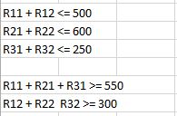
There are two constraints and one is related to location, and the other is related to work. Each location has maximum resources available, and Similarly, each work requires minimum resources to complete. Below is how we can visualize the problem.

for l1 in range(no_of_location):
    model += plp.lpSum(final_allocation[l1][w1] for w1 in range(no_of_work)) <= location_df['max_resource'].tolist()[l1]
for w2 in range(no_of_work):
    model += plp.lpSum(final_allocation[l2][w2] for l2 in range(no_of_location)) >= work_df['min_resource'].tolist()[w2]

Printing the model

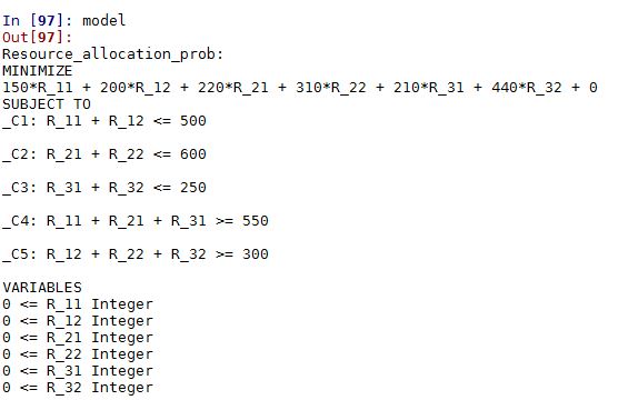
We will use a print statement to display the final model. We can print the model at intermediate steps to check how the model is being formed. The final model looks like below.

print(model)

I am running the model.

PuLP allows to choose solvers and formulate problems more naturally. The default solver used by PuLP is the COIN-OR Branch and Cut Solver (CBC)

model.solve()
status = plp.LpStatus[model.status]
print(status)

Checking optimal overall resource cost and the cost of each combination

print("Optimal overall resouce cost: ",str(plp.value(model.objective)))
for each in model.variables():
    print("Optimal cost of ", each, ": "+str(each.value()))

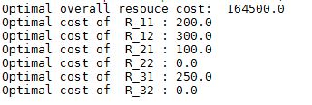
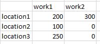
The below shows the optimal resource distribution. It is interesting to see how work2 can be handled by location1 alone. The results should always be cross-referenced with stakeholders to be more accurate. The model can be revisited according to business decisions.

Conclusion

I hope this article discussed the working of linear optimization problems that can be solved using the PuLP library. This article discussed pulp library, pulp models, import and export of models, the concept of optimization, and linear programming in brief. We can try them on other optimization problems and check results. It is always essential for any development to align with the business. When they are implemented on a large scale, they should get productive results. The solution should be implementable to create a meaningful impact. Happy coding!

Did you like my article on optimal resource allocation? Share in the comments below.

Head on to our blog, to read more articles.

Image sources: Author

The media shown in this article is not owned by Analytics Vidhya and are used at the Author’s discretion.