Pose Detection Using Computer Vision

This article was published as a part of the Data Science Blogathon.

Introduction

In this article, we will discuss some of the basic concepts related to Pose Detection. This article will cover a problem of the Computer Vision section of machine learning. In this article, we will gain knowledge of working with Image data and solve a very critical and real-world problem.

Before going in-depth, let’s list out what we will cover in this article.

Table of Contents

Let’s begin!

Introduction to Pose Detection

Pose Detection is a Computer Vision technique that predicts the tracks and location of a person or object. This is done by looking at the combination of the poses and the orientation of the given person or object.

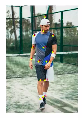
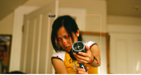
So, for a given image, we will first have to identify the person or the relevant object in the image, and then we will identify certain key points from the identified person or object.

Source:- Author

For a person, these key points can be the elbow knees, and so on. Combining these key points we can identify the pose of a person.

So, we’ll first identify the location of a person from the image and then we’ll detect key points for the person and finally combine these to determine the pose.

Now, there is a distinction between detecting one or multiple objects in an image or a video. So these two approaches can be referred to as single and multiple pose detection.

Single pose detection approaches detect and track one person or object while multiple detection approaches detect selecting multiple people or objects in the image with pose detection.

We are able to track an object or a person in real-world space at an incredibly granular level. This powerful capability opens up a wide range of possible applications also.

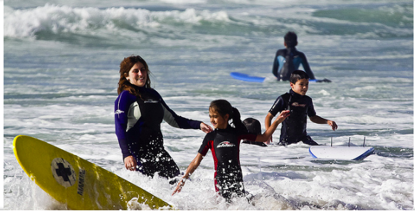
Let’s look at some of these interesting applications of pose detection. There are various online applications that use virtual yoga trainers and coaches to analyze the individual’s movements and poses. So we can use pose detection to determine whether the posture is correct or not.

It is widely used in the gaming industry as well. These systems track the user render their avatars in the game. In addition to performing tasks like gesture recognition or enabling the user to interact with the game.

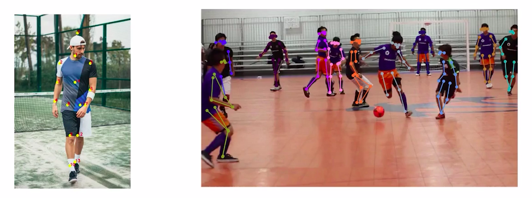
Source:- Author

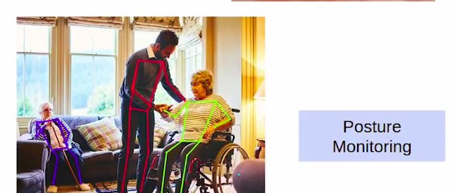
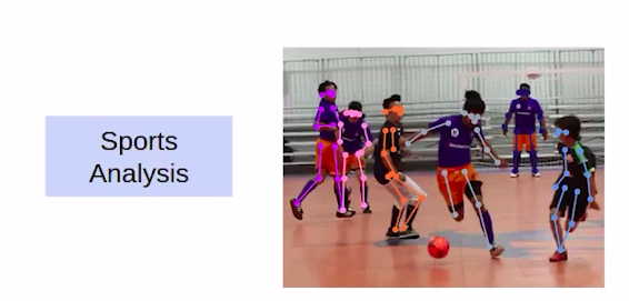
Pose detection can also be used for sports analysis to track the movement of players and can be used in the medical industry to monitor the posture of patients after physical therapy.

So these are some of the use cases and applications of pose detection.

Understanding the Problem Statement: COCO Keypoint Detection

In the previous section, we discussed an interesting use case of object detection which poses detection. We understood what pose detection is along with a few of its applications.

In this section, we’ll understand the problem statement that we have picked for our pose detection project. In this article, we’ll be working on the coco key point challenge where the objective is to determine the key points from the images.

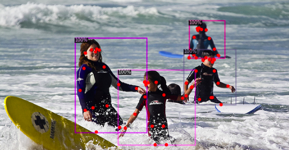
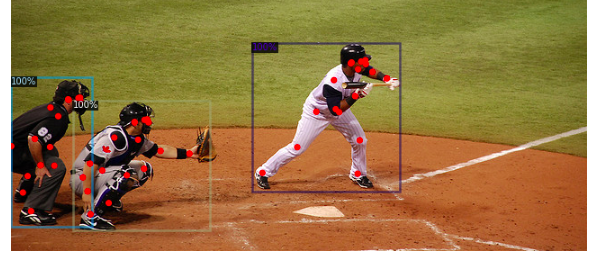
In this section, we’ll create a model which will take the images as inputs and predict two things:-
1. The bounding boxes around the person present in the image
2. The key points for the person.

Source:- Author

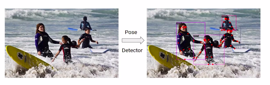
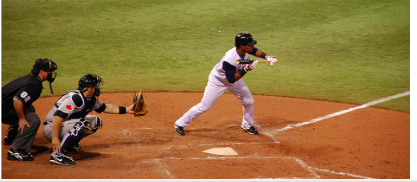
Here is another example if this is the input image for our model it should give us the output as shown here.

Source:- Author

So all the persons in the image are located and their key points are predicted. To train such a model, we will be working with the coco point data set.
Let’s have an overview of the dataset. In this dataset, we have around 59000 images separated into training and validation sets.

These images include around 156000 annotated people including a total of around 1.7 million key points.

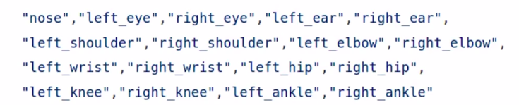
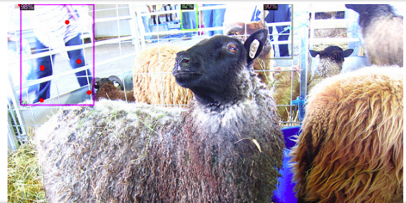
There can be 17 different types of key points that can be present in an image including the nose left eye right eye left ear right ear and so on so.

Source:- Author

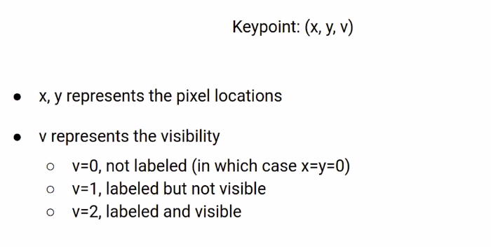
Each person in an image can have a maximum of 17 key points. Each key point is represented using these values x y and v where x and y represent the pixel location of the point and v represents the visibility of that particular key point.
if v is equal to 0 it means that the key point is not labeled or this particular key point is not present in the image.

If v is equal to 1 means that the key point is labeled but is not visible in the image.

If v is equal to 2 means that the key point is labeled and is visible.

 Source:- Author

So, this is all about the data set that we’ll be using to build our pose detection model.

To create our model will not use the entire cocoa data set. To train the model on the entire data set would require a huge amount of computational resources. So, we’ll take a small sample of the dataset.

we have already created a sample and you can download the data set that will be used from the link provided below.

Dataset link:- https://courses.analyticsvidhya.com/courses/take/Applied-Computer-Vision-using-Deep-Learning/downloads/14566628-dataset-coco-keypoints

We’ll be using the detectoron2 library to build a pose detection model. Since it provides an easier way to implement state-of-the-art object detection models.

Let’s look at the steps that will be followed to build our pose detection model.

1. Installing the dependencies like detecton2 library along with its prerequisites
2. We’ll load and pre-process the data set
3. We’ll define our model and train it.
4. Evaluate the model performance

So let’s move on to the next section and build our own pose detection model from scratch.

Building Your Own Pose Detection Model from scratch

Till now we have understood, what is a pose detection problem along with its applications. we also explored the coco keypoint dataset a bit which we’ll be using to build our pose detection model.

finally, we looked at the few steps that we’ll be following to build this model and a few of the steps that we have discussed in the above section.

So let’s start with

1. Installing the Dependencies

first of all, we are installing the 5.1 version of the “pyml” library which is required to run detectron2 smoothly.

Here we are installing the detectoron2 library.

!pip install pyyaml==5.1
# install detectron2:
!pip install detectron2==0.1.3 -f https://dl.fbaipublicfiles.com/
                    detectron2/wheels/cu101/torch1.5/index.html

2. Load the Dataset and Preprocess

Dataset link:-  https://courses.analyticsvidhya.com/courses/take/Applied-Computer-Vision-using-Deep-Learning/downloads/14566628-dataset-coco-keypoints

The data set is uploaded on the drive we’ll have to mount the drive first.

Once we have mounted the drive we can extract both the train and the validation images using the unzip command.

# mount drive
from google.colab import drive
drive.mount('drive/')

We are loading the images present in the training and the validation sets.

# extract files
!unzip 'drive/My Drive/pose_dataset/training_images.zip'
!unzip 'drive/My Drivea/pose_dataset/validation_images.zip'

We’ll use the glob library here which will give us the names of all the images in a folder. Hence importing glob first. Here creating an empty list name is train_images which will be used to store the training images.

After that, we are using a “for” loop and we are reading all the images present in the training set and appending them to the train image list. Similarly, we are storing the images for the validation set in a list named Val images.

from glob import glob
# for dealing with images
import cv2
# create lists
train_images  = []
# for each image
for i in glob('content/train2017/*.jpg'):    
    img=cv2.imread(i)
    #append image to list
    train_images.append(img)
# create lists
val_images  = []
# for each image
for i in glob('content/val2017/*.jpg'):    
    img=cv2.imread(i)    
    #append image to list
    val_images.append(img)

Once our dataset is ready the next step is to define our model and finally train it. So if you recall in order to use any data set in detectron2 we must first register this data set.  Hence we are registering the training data set here as train_data. we are also passing the location of the annotation files for the training set along with the path for the images.

from detectron2.data.datasets import register_coco_instances
register_coco_instances("train_data", {}, 'drive/My Drive/pose_dataset/
                person_keypoints_train2017.json',  "content/train2017/")

We are also registering metadata here and specifying the class as a person since we only have a portion of key points in the data set.

from detectron2.data import MetadataCatalog, DatasetCatalog
pose_metadata = MetadataCatalog.get("train_data").set(thing_classes=["person"])

Now, our dataset is registered. We’ll define the model in the next section code.

3. Train Model

We’ll be training our pose detection model from scratch using training images. So we’ll take the RCNN architecture for the keypoint detection task which is available in detectron2 and train it from scratch.

Here, we are importing a few functions from the detectron2 library which will help us to build and train our model. This model will be used to load the architectures of the model. Default trainer will be used to train our model and get_cfg will be used to get the configuration file for the model.

So first of all, we are defining the configuration instance as cfg and then we are defining the data set in the configuration file.

The training data is registered as train_data. we’ll use that here and keep the test data set empty for now next. We are loading the architectures for the RCNN model which is available in detectron2.

Finally, we are setting the threshold for detection as 0.7. Since we’ll also be detecting the bounding boxes.

# import some common detectron2 utilities
from detectron2 import model_zoo
from detectron2.engine import DefaultTrainer
from detectron2.config import get_cfg
# define configure instance
cfg = get_cfg()
cfg.DATASETS.TRAIN = ("train_data",)
cfg.DATASETS.TEST = ()
# Get a model specified by relative path under Detectron2’s official configs/ directory.
cfg.merge_from_file(model_zoo.get_config_file
                        ("COCO-Keypoints/keypoint_rcnn_X_101_32x8d_FPN_3x.yaml"))
# set threshold for this model
cfg.MODEL.ROI_HEADS.SCORE_THRESH_TEST = 0.7

Next, We are creating a directory to store the weights for the model to the make directory function is used. Here finally we are defining a few hyperparameters for our model.

import os
# create directory to save weights
os.makedirs(cfg.OUTPUT_DIR, exist_ok=True)

So the number of images per batch is set as 2, the learning rate is 0.001, the number of iterations is 2000, and the number of classes is 1.

# no. of images per batch
cfg.SOLVER.IMS_PER_BATCH = 2
# set base learning rate
cfg.SOLVER.BASE_LR = 0.001  
# no. of iterations 
cfg.SOLVER.MAX_ITER = 2000
# only has one class (person)
cfg.MODEL.ROI_HEADS.NUM_CLASSES = 1

Since we have only one person in the class so this completes our model architecture.

There are a few requirements for detectron2. It assumes that all the images, as well as the annotations, should be present in a folder named coco. So all images should be in a different folder and annotations should be in a separate folder. We are making those folders using the mkdir command. we have created a
folder data set and inside that, we have created a folder named coco.

Where we’ll move all the images and inside the coco folder we have created the annotations folder. where we’ll save the annotations.

!mkdir datasets
!mkdir datasets/coco
!mkdir datasets/coco/annotations

so here we are copying the annotation files for both the training and the validation sets using the cp command. So first we have to pass the location of the file that we wish to copy followed by where we want to copy that file.

!cp 'drive/My Drive/pose_dataset/person_keypoints_train2017.json' 
                                            'datasets/coco/annotations/'
!cp 'drive/My Drive/pose_dataset/person_keypoints_val2017.json' 
                                        'datasets/coco/annotations/'

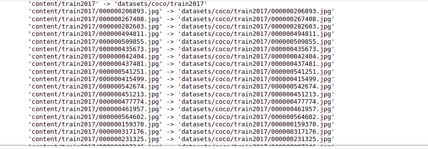
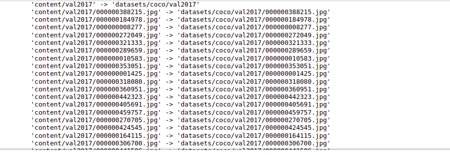
Next, we are copying the entire train2017 folder to the coco folder.

!cp -avr content/train2017 datasets/coco/

                           Source:- Author

Similarly, we’ll copy the val2017 folder as well.

!cp -avr content/val2017 datasets/coco/

                                                                                  Source:- Author

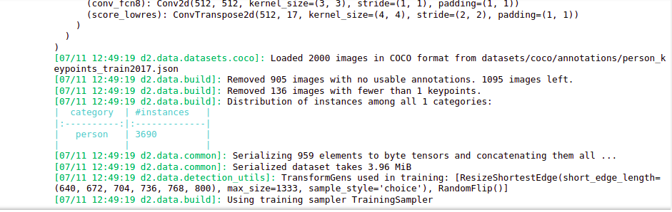
And now our model is ready and the dataset is in the correct folders as per the requirement of detectron2. So here we are defining the trainer using the default trainer which we have imported earlier and passing the cfg file inside it.

# Create trainer
trainer = DefaultTrainer(cfg)

The output is:-

                                                                                      Source:- Author

Here is the architecture for our model and our model has found 3690 instances of people in the training data set.

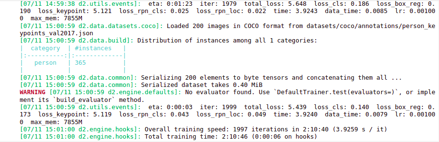
Next, we are training the model and setting the resume as false because we want to start the training from scratch. So using the dot train function we are training the model.

trainer.resume_or_load(resume=False)
# train the model
trainer.train()

The output is:-

                                                                                        Source:-Author

here the training process initially the loss is around 9.6 and as the training progresses the loss reduces to 5.6.

This model took two hours to train for 2000 iterations. Now that our model is trained. The next section will evaluate the performance.

4. Evaluate the Performance

let us evaluate the performance of the validation set. so we are first registering the validation dataset as validation_data and its metadata similar. how we registered the training data.

register_coco_instances("validation_data", {},
        'drive/My Drive/pose_dataset/person_keypoints_val2017.json', "content/val2017/")
pose_metadata = MetadataCatalog.get("validation_data").set(thing_classes=["person"])

Now we are defining the weights that were saved during the training. we are keeping the threshold as 0.5 here. We are defining the test set in the configuration file as validation_data.

# load the final weights
cfg.MODEL.WEIGHTS = os.path.join(cfg.OUTPUT_DIR, "model_final.pth")
# set the testing threshold for this model
cfg.MODEL.ROI_HEADS.SCORE_THRESH_TEST = 0.5
# List of the dataset names for validation. Must be registered in DatasetCatalog
cfg.DATASETS.TEST = ("validation_data", )

Next, we are defining the default predictor of detectron2 and passing the configuration file which will be used to get the predictions.

# set up predictor
from detectron2.engine import DefaultPredictor
# Create a simple end-to-end predictor with the given config
# that runs on single device for a single input image.
predictor = DefaultPredictor(cfg)

After that, we’ll use the visualizer library in order to visualize some of the images from the data. So random will be used to randomly pick the images for visualization.

The visualizer function of detectron2 will be used to visualize the predictions. The cv2_imshow will be used to display the images.

Now using a for loop we are taking images randomly from the train set and then making the predictions for these images using the predictor. We have already defined it previously.

Now we are defining the visualizer and using the draw_instance_predictions and we are drawing the predictions on these images.

finally, here we are visualizing the output. So here are a few predictions as per our model.

import random
#for drawing predictions on images
from detectron2.utils.visualizer import Visualizer
#to display an image
from google.colab.patches import cv2_imshow
#randomly select images
for img in random.sample(train_images,5):      
    #make predictions
    outputs = predictor(img)
    # Use `Visualizer` to draw the predictions on the image.
    v = Visualizer(img[:, :, ::-1], metadata = pose_metadata, scale=1)
    #draw prediction on image
    v = v.draw_instance_predictions(outputs["instances"].to("cpu"))
    #display image
    cv2_imshow(v.get_image()[:, :, ::-1])

In the first image, the model has identified the person as well as the key points. Similarly, for the other images, you can see that the model has accurately identified the people and the key points on these outputs.

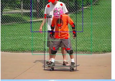
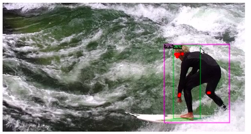
                                                                                Source:- Author

Let us now look at the overall performance of the model on the validation set. So we are importing a few helper functions. Here This will help us evaluate the performance. First of all, we are defining the predictor then we are defining the evaluator using the coco evaluator function and then loading the validation images. We are defining the data loader using build_detection_ test_loader. Finally, we are taking the inferences on the validation set using inference on the data set function.

# test evaluation
from detectron2.data import build_detection_test_loader
from detectron2.evaluation import COCOEvaluator, inference_on_dataset
predictor = DefaultPredictor(cfg)
evaluator = COCOEvaluator("validation_data", cfg, False, output_dir="./output/")
val_loader = build_detection_test_loader(cfg, "validation_data")
inference_on_dataset(trainer.model, val_loader, evaluator)

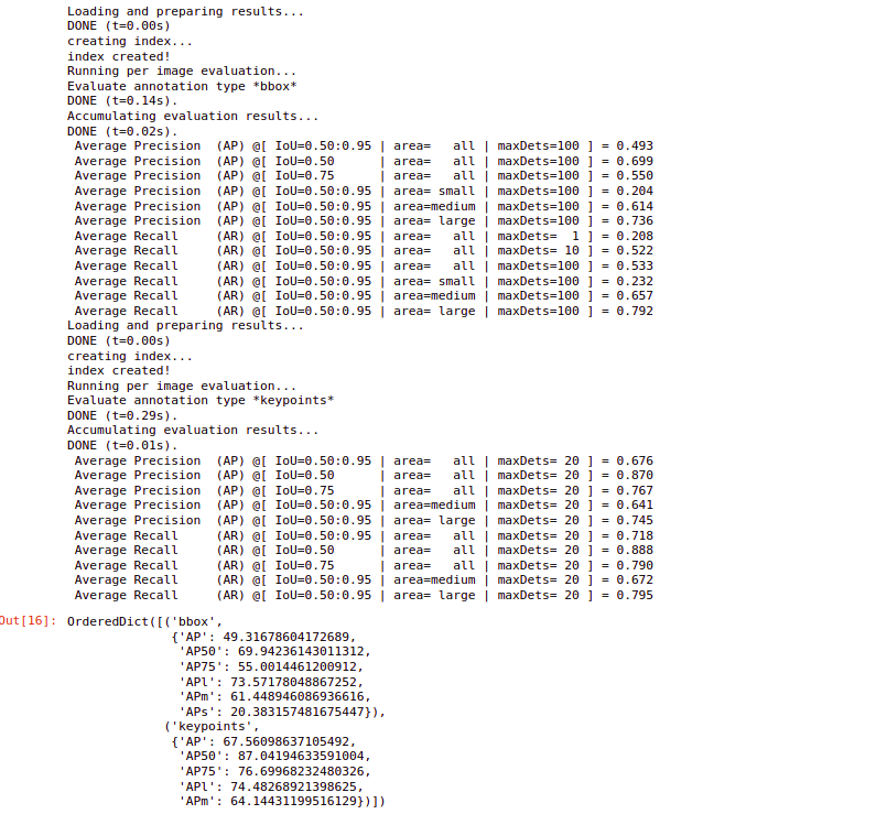
and here are the results.

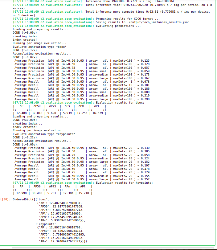
                                                                                           Source:- Author

So we have the performance for both the bounding boxes as well as the key points the average precision at an iou of 0.5 is around 38 for key points. This performance is quite less. There are majorly two reasons for this:-

1. first of all we did not take the entire training data set to train the model. Here we only retrained the model for 2000 iterations.

2. we can increase the number of training images and the iterations and the performance can also be improved.

so in the next section, we’ll use a pre-trained model which is trained on the entire training set of the coco keypoint dataset for a very large number of iterations and we’ll see if that improves the model performance.

Using a Pre-Trained Model to build a Pose Detection Model

In the last section, we trained a pose detection model from scratch using the detectoron2 library.

Now in this section, we are going to use a pre-trained model which has been trained on a larger amount of data set and for more number iterations to see how the model will perform.

1. Installing the Dependencies

So first of all we are loading the dependencies so we have loaded the 5.1 version of the pyml library. we have also installed the detectron2 library.

!pip install pyyaml==5.1
# install detectron2:
!pip install detectron2==0.1.3 -f https://dl.fbaipublicfiles.com/detectron2
                /wheels/cu101/torch1.5/index.html

2. Load the Dataset and Preprocess

Now we are loading the dataset from the drive. So we have to first mount the drive and then extract the files from the drives.

# mount drive
from google.colab import drive
drive.mount('drive/')

So we are extracting only our validation images because we do not want to train the model.

# extract files
!unzip 'drive/My Drive/pose_dataset/validation_images.zip'

In order to read the images and store the images, we will be using the glob library and the cv2 for reading and visualizing the images. So first we are using glob in order to store all the image names in a list.

Once all the image names are stored, we are going to use the imread function in order to read these images one by one and store them in the list.

from glob import glob
# for dealing with images
import cv2
# create lists
images  = []
# for each image
for i in glob('content/val2017/*.jpg'):    
    img=cv2.imread(i)
    #append image to list
    images.append(img)

Now we are using the detectoron2 library here to load the pre-trained model. first of all, we are going to use the model zoo which will have pre-trained models. After that, we are going to use the default predictor for making the predictions on our validation set and get cfg in order to load the default configuration file.

so here we have first created a class instance of cfg and then we are taking the selected model which will be our RCNN model which has been trained on the coco keypoint dataset and loading this model.

3. Train Model

Now we are going to use the pre-trained model. we’ll also load the weights and define the weights as the weights for this model.

Here we have set a threshold value and then we have created a predictor using the default predictor and passed it in our cfg file.

# import some common detectron2 utilities
# to obtain pretrained models
from detectron2 import model_zoo
# set up predictor
from detectron2.engine import DefaultPredictor
# set config
from detectron2.config import get_cfg
# define configure instance
cfg = get_cfg()
# Get a model specified by relative path under Detectron2’s official configs/ directory.
cfg.merge_from_file(model_zoo.get_config_file
                ("COCO-Keypoints/keypoint_rcnn_R_101_FPN_3x.yaml"))
# download pretrained model 
cfg.MODEL.WEIGHTS = model_zoo.get_checkpoint_url
                    ("COCO-Keypoints/keypoint_rcnn_R_101_FPN_3x.yaml")
# set threshold for this model
cfg.MODEL.ROI_HEADS.SCORE_THRESH_TEST = 0.8

# Create predictor
predictor = DefaultPredictor(cfg)

Now before we go ahead we’ll have to register the data set so we are registering our validation data here and then also defining the metadata catalog. Now we have to define the class which is a person here.

from detectron2.data.datasets import register_coco_instances
register_coco_instances("validation_data", {}, 'drive/My Drive/pose_dataset
        /validation_annotation.json', "content/val2017/")

from detectron2.data import MetadataCatalog
pose_metadata = MetadataCatalog.get("validation_data").set(thing_classes=["person"])

We have made the predictions using the model on the randomly selected images and then we are plotting the predictions on the images or drawing the predictions on the images and then displaying the images.

import random
#for drawing predictions on images
from detectron2.utils.visualizer import Visualizer
#to obtain metadata
from detectron2.data import MetadataCatalog
#to display an image
from google.colab.patches import cv2_imshow
#randomly select images
for img in random.sample(images,5):      
    #make predictions
    outputs = predictor(img)
    # Use `Visualizer` to draw the predictions on the image.
    v = Visualizer(img[:, :, ::-1], metadata = pose_metadata, scale=1)
    #draw prediction on image
    v = v.draw_instance_predictions(outputs["instances"].to("cpu"))
    #display image
    cv2_imshow(v.get_image()[:, :, ::-1])
    cv2_imshow(img)

 

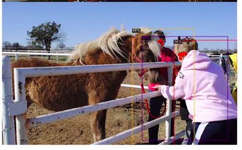
So you can see here that the portions in the picture are correctly identified or located and the key points are also marked for all of these images. So this is the predicted image and this was our original image. similarly, you can see a couple more examples so this is the predicted image and the original image.

Source:-Author

4. Evaluate the Performance

Now in order to evaluate our model as we saw before we are going to use a detectoron2. To evaluate and import the coco evaluator. So first of all we’ll make the predictions using the default predictor, and use the coco evaluator in order to evaluate the predictions on the validation data,  and here are the inferences.

#test evaluation
from detectron2.data import build_detection_test_loader
from detectron2.evaluation import COCOEvaluator, inference_on_dataset
predictor = DefaultPredictor(cfg)
evaluator = COCOEvaluator("validation_data", cfg, False, output_dir="./output/")
val_loader = build_detection_test_loader(cfg, "validation_data")
inference_on_dataset(predictor.model, val_loader, evaluator)

 

Source:-Author

So, we can see in the above image, the average precision of 0.5 RUU for the key points is 87. This is much better than the model that we have trained. Mainly because this model has been trained on a huge data set, and for a large number of iterations. So you can see that the model performance has significantly improved.

Conclusion

so we are going to use pose detection in order to classify the images of sports let’s go to the next article and we’ll discuss more to more this in the next article.

Thank you.

About the Author

Hi, I am Kajal Kumari. have completed my Master’s from IIT(ISM) Dhanbad in Computer Science & Engineering. As of now, I am working as Machine Learning Engineer in Hyderabad. Here is my Linkedin if you want to connect with me.

End Notes

Thanks for reading!

I hope that you have enjoyed the article. If you like it, share it with your friends also. Something not mentioned or want to share your thoughts? Feel free to comment below And I’ll get back to you.

If you want to read my previous blogs, you can read Previous DJodhpurata Science Blog posts from here.

The media shown in this article is not owned by Analytics Vidhya and are used at the Author’s discretion.

kajal

Hi, I am Kajal Kumari. have completed my Master’s from IIT(ISM) Dhanbad in Computer Science & Engineering. As of now, I am working as Machine Learning Engineer in Hyderabad.
hope that you have enjoyed the article. If you like it, share it with your friends also. Please feel free to comment if you have any thoughts that can improve my article writing.

If you want to read my previous blogs, you can read Previous Data Science Blog posts here. Connect with me