A Basic Introduction to Object Detection

Introduction

Computer vision has advanced considerably but is still challenged in matching the precision of human perception. This article belongs to computer vision. Here we will learn from scratch. It can be challenging for beginners to distinguish between different related computer vision tasks.

Humans can easily detect and identify object detection using machine learning present in an image. The human visual system is fast and accurate and can perform complex tasks like identifying multiple objects and detecting obstacles with little conscious thought. With the availability of large amounts of data, faster GPUs, and better algorithms, we can now easily train computers to detect and classify multiple objects within an image with high accuracy.

With this kind of identification and localization, object detection can be used to count objects in a scene and determine and track their precise locations, all while accurately labeling them.

In this guide, you’ll find answers to all of those questions and more. Whether you’re an experienced machine learning engineer considering implementation, a developer wanting to learn more, or a product manager looking to explore what’s possible with computer vision and object detection using machine learning, this article is for you.

Let’s Start.

This article was published as a part of the Data Science Blogathon.

What is Object Detection?

Object detection, within computer vision, involves identifying objects within images or videos. These algorithms commonly rely on machine learning or deep learning methods to generate valuable outcomes.

Now let’s simplify this statement a bit with the help of the below image.

So instead of classifying, which type of dog is present in these images, we have to actually locate a dog in the image.  That is, I have to find out where is the dog present in the image? Is it at the center or at the bottom left? And so on. Now the next question comes into the human mind, how can we do that? So let’s start.

Well, we can create a box around the dog that is present in the image and specify the x and y coordinates of this box.

for now, consider that the location of the object in the image can be represented as coordinates of these boxes. So this box around the object in the image is formally known as a bounding box. Now, this becomes an image localization problem where we are given a set of images and we have to identify where is the object present in the image.

Note that here we have a single class. what if we have multiple classes?

Example:

In this image, we have to locate the objects in the image but note that all the objects are not dogs. Here we have a dog and a car. So we not only have to locate the objects in the image but also classify the located object as a dog or Car. So this becomes an object detection problem.

This article will also discuss a few points regarding image classification also. we will discuss image classification v/s object detection.

In the case of object detection problems, we have to classify the objects in the image and also locate where these objects are present in the image. But the image classification problem had only one task where we had to classify the objects in the image.

So for the one example, you can see below the image that we have been working on in the first case, we predict only the target class, and such tasks are known as image classification problems. While in the second case, along with predicting the target class, we also have to find the bounding box which denotes the location of the object. This is all

This is all about the object detection using machine learning problem. So broadly we have three tasks for object detection problems:

• To identify if there is an object present in the image,
• Where is this object located,
• What is this object?

So you can see the below image.

Specific to this example, we have an object in the image. We can create a bounding box around the object and this object is an emergency vehicle.

Now the object detection problem can also be divided into multiple categories.

First is the case when you have images that have only one object. That is you can have 1000 images in the data set, and all of these images will have only one object. And if all these objects belong to a single class, that is all the objects are cars, then this will be an image localization problem. That is you already know what class these objects belong to, you only have to locate where these objects are present in the image.

Another problem could be where you are provided with multiple images, and within each of these images, you have multiple objects. Also, these objects can be of the same class, or another problem can be that these objects are of different classes.

So in case you have multiple objects in the image and all of the objects are of different classes. you would have to not only locate the objects but also classify these objects.

The next section will discuss the problem statement for object detection.

Why Object Detection Matters?

• Safety: It helps keep us safe by spotting dangers and intruders.
• Driving: It’s crucial for self-driving cars to avoid accidents.
• Shopping: It helps stores manage products and understand customers.
• Healthcare: Doctors use it to find diseases early in medical images.
• Manufacturing: It ensures products are made correctly in factories.

How object detection Works?

Here Object Detection Works:

• Looking at the Picture: Imagine a computer looking at a picture.
• Finding Clues: The computer looks for clues like shapes, colors, and patterns in the picture.
• Guessing What’s There: Based on those clues, it makes guesses about what might be in the picture.
• Checking the Guesses: It checks each guess by comparing it to things it already knows.
• Drawing Boxes: If it’s pretty sure about something, it draws a box around it to show where it thinks the object is.
• Making Sure: Finally, it double-checks its guesses to make sure it got things right and fix any mistakes

Training Data For Object Detection

Dataset link:- Click Here

In the last section, we discussed the object detection using deep learning problem and how it is different from a classification problem. We also discussed that
there are broadly three tasks for an object detection using machine learning problem.

Now in this section, we’ll understand what the data would look like for an object detection using deep learning task.

So, let’s first take an example from the classification problem. In the below image, we have an input image and a target class against each of these input images.

Now, suppose the task at hand is to detect the cars in the images. So in that case will not only have an input image but along with a target variable that has the bounding box that denotes the location of the object in the image.

So, in this case, this target variable has five values the value p denotes the probability of an object being in the above image whereas the four values Xmin, Ymin, Xmax, and Ymax denote the coordinates of the bounding box. Let us understand how these coordinate values are calculated.

So, consider the x-axis and y-axis above the image there. In that case, the Xmin and Ymin will be the top left corner of the bounding box, and Xmax and Ymax will be the bottom right corner of the bounding box. Now, note that the target variable(P) answers only two questions?

1. Is there an object present in the image?

Answer:- If an object is not present then p will be zero and when there is an object present in the image p will be one.

2. if an object is present in the image where is the object located?

Answer:- You can find the object location using the coordinates of the bounding box.

In case all the images have a single class that is just a car. What happens when there are more classes? In that case, this is what the target variable would look like.

So, if you have two classes which are an emergency vehicle and a non-emergency vehicle, you’ll have two additional values c1 and c2 denoting which class does the object present in the above image belong.

So if we consider this example, we have the probability of an object present in the image as one. We have the given Xmin, Ymin, Xmax, and Ymax as the coordinates of the bounding box. And then we have c1 is equal to 1 since this is an emergency vehicle and c2 would be 0 because of a non-emergency vehicle.

Now, this is what the training data should look like in the above image.

let’s say we build a model and get some predictions from the model, this is a possible output that you can get from a model. The probability that an object is present in this predicted bounding box is given as 0.8. you have the coordinates of this blue bounding box, which is the predicted bounding box which is (40,20) and (210,180), and then finally the class value of c1 and c2.

So now we understand what is an object detection using deep learning problem and what the training data for an object detection problem would look like.

Before moving into depth, we need to know a few concepts regarding images such that:

• How to do Bounding Box Evaluation?
• How to calculate IoU?
• Evaluation Metric – mean Average Precision

Let’s start with the first one is Bounding Box Evaluation.

Bounding Box Evaluation – Intersection over Union (IoU)

In this section, we are going to discuss a very interesting concept, which is the intersection over the union(IoU). And we are going to use this, in order to determine the target variable for the individual patches that we have created.

So, consider the following scenario. Here we have two bounding boxes, box1 and box2. Now if I ask you which of these two boxes is more accurate, the obvious answer is box1.

Why? Because it has a major region of the WBC and has correctly detected the WBC. But how can we find this out mathematically?

So, compare the actual, and the predicted bounding boxes. if we are able to find out the overlap of the actual, and the predicted bounding box, we will be able to make a decision as to which bounding box is a better prediction.

So the bounding box that has a higher overlap with the actual bounding box is a better prediction. Now, this overlap is called the area of intersection for this first box, which is box1. We can say that the area of intersection is about 70% of the actual bounding box.

Whereas, if you consider box2, the area of intersection of the second bounding box, and the actual bounding box is about 20 %.

So we can say that of these two bounding boxes obviously, box1 is a better prediction.

But having the area of intersection alone is not enough. Why? let’s find out.

Scenarios:- 1

Let’s consider another example suppose we have created multiple bounding boxes or patches of different sizes.

Here, the intersection of the left bounding box is certainly 100% whereas, in the second image, the intersection of this predicted bounding box, or this particular patch is just 70%. So at this stage, would you say that the bounding box on the left is a better prediction? obviously not. The bounding box on the right is more accurate.

So, to deal with such scenarios, we also consider the area of union, which is the patch area, as well as the actual bounding box area.

So, higher this area of union(blue region) we can say that less accurate will be the predicted bounding box, or the particular patch. Now, this is known as intersection over the union(IoU).

So here we have the formula for the intersection over union, which is the area of the intersection divided by the area of union.

Now, what would be the range of intersection? Let’s consider some extreme scenarios.

So in case we have our actual bounding box and predicted bounding box, and both of these have no overlap at all, in that case, the area of the intersection will be zero, whereas the area of union will be the sum of the area of this patch. So, overall the IoU would be zero.

Scenario:- 2

Another possible scenario could be when both the predicted bounding box and the actual bounding box completely overlap.

In that case, the area of the intersection will be equal to this overlap, and the area of union will also be the same. Since the numerator and the denominator would be the same in this case, the IoU would be 1.

So, basically, the range of IoU or intersection over union is between 0 and 1.

Now we often consider a threshold, in order to identify if the predicted bounding box is the right prediction. So let’s say if the IoU is greater than a threshold which can be, let’s say 0.5 or 0.6. In that case, we will consider that the actual bounding box and the predicted bounding box are quite similar.

Whereas if the IoU is less than a particular threshold, we’ll say that
the predicted bounding box is nothing close to the actual bounding box.

Example:

We have to identify the target or whether a WBC is present in either of these patches.

So we can consider the intersection over union for a particular threshold. Let’s say if the Iou value is greater than 0.5, we’ll classify that the particular patch has a WBC and if the IoU is less than this particular threshold we can say that the particular patch does not have the WBC.

We are obviously free to set this threshold at our own end.

Now apart from using “IoU”, It Can be Used as:-

• For selecting the best bounding box
• As an evaluation Metric

Since if the intersection over union is high, then the predicted bounding boxes are close to the actual bounding box, and we can say that the model is performing well.

Hence “IoU” can also be used as an evaluation metric now in the next section we’ll learn how to calculate the IoU for bounding boxes.

Calculation IOU

In this section, we’ll learn how to calculate the IoU value or the intersection over the union.

This will also be helpful to understand the code for the intersection over the union in the notebook. So in the last section, we discussed that in order to calculate the IoU value. We need the area of intersection as well as the area of union.

Now the question is, how do we find out these two values? So to find out the area of intersection, we need the area of this blue box. And we can calculate that using the coordinates for this blue box.

So the coordinates will be Xmin, Ymin, Xmax and, Ymax using these coordinates values will be easily able to calculate the area of intersection. So let’s focus on determining the value of Xmin here.

In order to find out the value of Xmin, we are going to use the Xmin values for these two bounding boxes, which are represented as X1min and X2min.

Now, as you can see above the diagram, the Xmin for this blue bounding box is simply equivalent to X2min. We can also say that the Xmin for this blue box will always be the maximum value out of these two values X1min and X2min.

Similarly, in Order to Find Out the Value:

Xmax for this blue bounding box, we are going to compare the values X1max and X2max. We can see that the Xmax for this blue bounding box is equivalent to X1max. It can also be written as the minimum of X1max and X2max.

Similarly in order to find out the value for Ymin and Ymax. We are going to compare the Y1min and Y2min, and Y1max and Y2max. The value of Ymin will simply be the maximum of Y1 minimum and Y2 minimum which you can see here.

And similarly, the

Ymax will be the minimum of Y1max and Y2max.

Now once we have these four values which are Xmin, Ymin, Xmax, and Ymax.

We can calculate the area of intersection by multiplying the length and the width of this rectangle, which is the blue rectangle right here.

So to find out the length, we are going to subtract Xmax and Xmin. And to find out the height, or the width here, we are going to find the difference between Ymax and Ymin. Once we have the length and width, the area of the intersection will simply be the length multiplied by width. So now we understand how to calculate the area of intersection.

Area of union

Next, the focus is on calculating the area of union. So in order to calculate the area of union, we are going to use the co-ordinate values of these two bounding boxes which are the green bounding box and the red bounding box.

So first of all we’ll have to find out the area of box1 which is the length into a width of this green bounding box, or this green shaded
region.

Now note that, when we are calculating the areas of box1 and box2, we are actually counting this blue shaded region twice. So this is a part of the green rectangle as well as the red rectangle. Since this part is counted twice we’ll have to subtract it once, in order to get the area of union.

So the area of union finally will be the summation of the area of box1 and the area of box2 after that have to subtract the intersection area since this has been counted twice.

So now we have the area of intersection for two bounding boxes and also have the area of union for two bounding boxes. Now we can simply
calculate the intersection over union as the area of the intersection divided by the area of union.

Now in the next section, we are going to understand the Evaluation of metrics.

Evaluation Metric – mean Average Precision

Now, we are going to discuss some popularly used evaluation metrics for object detection using deep learning.

Evaluation Metrics for Objection Detection:-

• Intersection over union(IoU)
• Mean Average Precision(mAP)

So we have previously discussed the intersection over the union and How it can be used to evaluate the model performance by comparing the predicted bounding boxes with the actual bounding boxes. Another popularly used metric is mean average precision.

So in this section, we will understand what is mean, average precision and how it can be used.

 Mean, Average Precision

Now, I’m sure you’re familiar with the metric precision, which simply takes into account the number of true positives, and is divided by the true positives and false positives. So this is basically the actual positive values upon the predicted positive values.

 Now, let’s take an example to understand, how precision is calculated. So let’s say if we have a set of bounding box predictions. Along with that, we have the IoU score which we calculated by comparing these bounding box predictions with the actual bounding boxes.

Now, let’s say we have a threshold of 0.5.

So in that case, we would be able to classify these predictions as true positives and false positives. Once we have the total number of true positives and false positives, we would be able to calculate the precision rate. So the precision, in this case, is 0.6.

Now there’s another metric which is average precision. So average precision basically calculates the average of the precision values across the data.

So let’s understand this with an example of how it works that will give you a better idea of what average precision is.

Example:

So we saw that in this above image example, we have five bounding boxes with their IoU scores, and based on the IoU score we can define if this bounding box is a true positive or a false positive. Now, we calculate the precision for this particular scenario where we are only considering the bounding box1.

Let’s break down object detection for machine learning. We’re talking about how well a system can spot objects in images. Now, let’s get into the numbers. Imagine we’re looking at the first box around an object. If it’s correctly identified (a true positive), we give it a score of one.

The bottom number of our precision calculation is the total of true positives and false positives. In this case, it’s also one. So, the precision for this box is one. Even if there’s a false positive, we keep the precision value the same. We repeat this process for the other boxes. Say we’re checking the third box and find a true positive. Now, we have two true positives in total. The sum of true positives and false positives is three. So, the precision at this point is calculated as 2 divided by 3, which equals 0.66.

Similarly, we would calculate for all the bounding boxes. So for the fourth bounding box, we’ll have three true positives and a total number of 4 true positives and false positives.  Hence, this value would be 3 by 4 or 0.75.

Once we calculate all of these precision values for the bounding boxes, we are going to take an average of these precision values, which are also known as interpolated precision, and we take an average here to calculate the average precision.

Mean Average Precision

Now, mean average precision is simply calculated across all the classes.

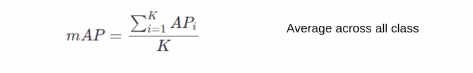
So let’s say we have multiple classes or let’s say we have k classes, then for each individual class, we’ll calculate this average precision, and take an average across all the classes. This would give you the mean average precision. So this is how mean average precision is calculated for the object detection problems and is used as an evaluation metric to compare and evaluate the performance of these object detectors.

Conclusion

The theory and fundamentals of object detection are critical for solving the business challenge and developing the necessary model. When it comes to working with image data, the most difficult task is figuring out how to detect objects from images that can be applied to the model. While working on image data you have to analyze a few tasks such as object detection, bounding box, calculating IoU value, Evaluation metric.I hope the articles helped you understand how to deal with image data, how to detect objects from images, we are going to use this technique, and apply it in a few domains such as the medical, sports analysis domain.

The media shown in this article is not owned by Analytics Vidhya and are used at the Author’s discretion.

Frequently Asked Questions

Kajal Kumari 06 Jun 2024