This article was published as a part of the Data Science Blogathon.
Introduction
Pose Detection is a subset of the Computer Vision (CV) technique that predicts the tracks and location of a person or object. This is done by looking at the combination of the poses and the direction of the given person or object.
This article is an ongoing part of a blog that I have already written.
Please check out the below link to have a better understanding of Pose Detection.
Blog Link: Analytics Community | Analytics Discussions | Big Data Discussion (analyticsvidhya.com)
Objective
Earlier we got a better understanding of Pose Detection where we built a model using a pre-trained model. There are many interesting applications and use cases of pose detection. Now, in this article, we’ll discuss one such interesting application and build a model to solve that problem.
The objective of this article is to build a model that can classify the cricket shots using the pose of a player. For this, an image will be input into the model. It will detect the pose of the person in the image and then using the pose that was detected, we will classify what type of shot it was.
Table of Contents
1. Install Dependencies
2. Load and pre-process the data
3. Data Augmentation
4. Detecting pose using detectron2
5. Classifying cricket shot using pose of a player
6. Evaluating model performance
Install Dependencies for Cricket Shot Classification
!pip install pyyaml==5.1
# install detectron2:
!pip install detectron2==0.1.3 -f
     https://dl.fbaipublicfiles.com/detectron2/wheels/cu101/torch1.5/index.html
Load and Pre-Process the data for Cricket Shot Classification
We are going to load the dataset which is saved on the drive. So for that, we’ll mount the drive first after that we’ll extract the short zip file.
# mount drive
from google.colab import drive
drive.mount('drive/')
The short zip file contains the images for the different types of shots. Next, we are getting the names of the folders which are the classes or different types of shots.
# extract files
!unzip 'drive/My Drive/shot.zip'
Next, we are doing this using the list ERR function of the OS library. Here we are printing the folder names that we have so we have the four folders which are pull, cut, drive and sweep.
import os
# specify path
path='shot/'
# list down the folders
folders = os.listdir(path)
print(folders)
Output:- [‘pull’, ‘cut’, ‘drive’, ‘sweep’]
Next, we are reading all the images and stored them in a list named images. WWe will also be storing the labels in a list which basically is the class for each image. This class will be nothing but the name of the folder in which the image has been stored. You’re already familiar with the process that we are going to go through each folder and read the images one by one and append them in the created list.
# for dealing with images
import cv2
# create lists
images  = []
labels  = []
# for each folder
for folder in folders:
    # list down image names
    names=os.listdir(path+folder)
    # for each image
    for name in names:
        # read an image
        img=cv2.imread(path+folder+'/'+name)
        # append image to list
        images.append(img)
        # append folder name (type of shot) to list
        labels.append(folder)
Let’s quickly check the number of images using the length function. We can observe that there are 290 images.
# number of images
len(images)
Output:- 290
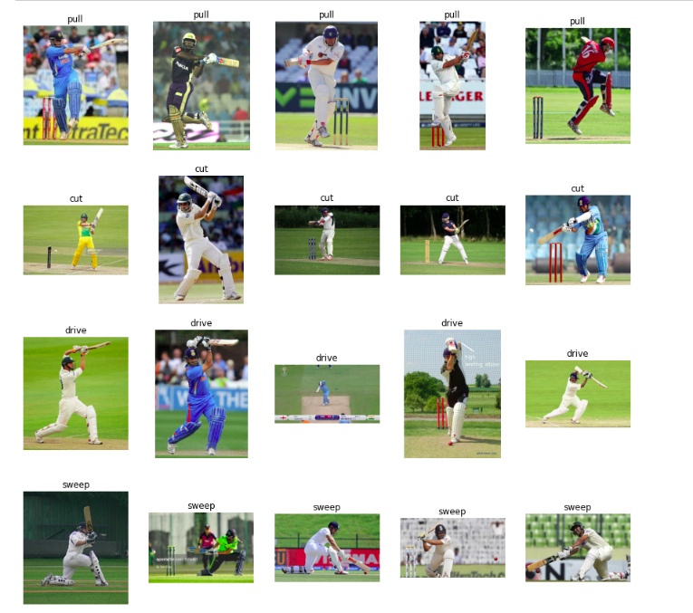
Now here we are visualizing a few images from the data set. So for each type of shot. We are plotting five images randomly. We will use the matplotlib to visualize the images. The random function will be used to randomly select the images.
We are going to create a subplot with four rows for the four different classes and five columns for the five examples. Next for each class, we’ll randomly pick five images and read the images using the cv2.imread function. Once You read the image, you can convert these images into RGB format and visualize these images.
# visualization library
import matplotlib.pyplot as plt
# for randomness
import random
# create subplots with 4 rows and 5 columns
fig, ax = plt.subplots(nrows=4, ncols=5, figsize=(15,15))
# randomly display 5 images for each shot for each folder
for i in range(len(folders)):
    # read image names
    names=os.listdir(path+folders[i])
    # randomly select 5 image names
    names= random.sample(names, 5)
    # for each image
    for j in range(len(names)):
      # read an image
      img = cv2.imread(path+ folders[i]+ '/' +names[j])
      # convert BGR to RGB
      img = cv2.cvtColor(img, cv2.COLOR_BGR2RGB)
      # display image
      ax[i, j].imshow(img)
      # set folder name as title
      ax[i, j].set_title(folders[i])
      # Turn off axis
      ax[i, j].axis('off')
Source:- Author
So, here you can see are a few examples of the images that we have taken from the dataset. Now since we have less number of images in the training set. We’ll use the data augmentation techniques to increase our training size.
Data Augmentation
To increase our training size so we’ll flip the images horizontally and this will help us with two things first of all the players can be both right-handed and left-handed so by flipping the images. It will make our model more generalized. It will also increase the number of images for training.
So here we are creating an empty list to store the augmented images and their corresponding labels for each image in the dataset.
We are flipping it using the flip function of cv2 and then we are appending it to the list.
# image augmentation
aug_images=[]
aug_labels=[]
# for each image in training data
for idx in range(len(images)):
  # fetch an image and label
  img  = images[idx]
  label= labels[idx]
  # flip an image
  img_flip = cv2.flip(img, 1)
  # append augmented image to list
  aug_images.append(img_flip)
  # append label to list
  aug_labels.append(label)
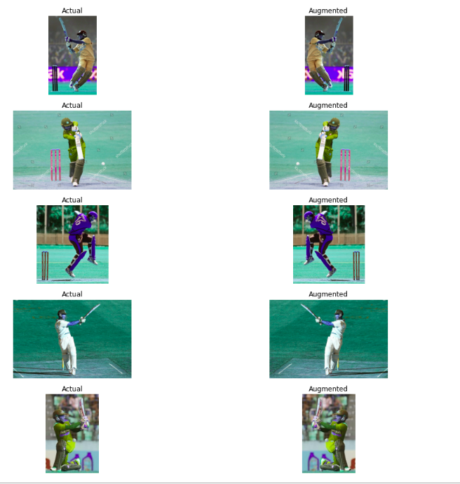
Next, we are going to visualize a few augmented images along with the original images.
So we are randomly picking five images. Also, we are creating a subplot to visualize like before we did. We are first plotting the actual image and then its augmented version.
So here we can see that using data augmentation for flipping the images the type of shot does not change. A pull shot is going to be a pull shot even if we rotate the image horizontally.
# display actual and augmented image for sample images
# create indices
ind = range(len(aug_images))
# randomly sample indices
ind = random.sample(ind, 5)
# create subplots with 5 rows and 2 columns
fig, ax = plt.subplots(nrows=5, ncols=2, figsize=(15,15))
# for each row
for row in range(5):
  # for each column
  for col in range(2):
    # first column for actual image
    if col==0:
      # display actual image
      ax[row, col].imshow(images[ ind[row] ] )
      # set title
      ax[row, col].set_title('Actual')
      # Turn off axis
      ax[row, col].axis('off')
    # second column for augmented image
    else:
      # display augmented image
      ax[row, col].imshow(aug_images[ ind[row] ] )
      # set title
      ax[row, col].set_title('Augmented')
      # Turn off axis
      ax[row, col].axis('off')
Source:- Author
Now we are combining the actual and the augmented images and checking the number of images.
# combine actual and augmented images & labels
images = images + aug_images
labels = labels + aug_labels
# number of images
len(images)
Output:- 580
Detecting pose using detectron2
Now we have 580 images including both the actual and the augmented images for training. Now our data set is ready. Next, we’ll detect the pose of the players in all of these images using detectron2.
So we will use a pre-trained model present in detectron2 to detect these poses here. We are defining the model and a few libraries. We are defining the model architecture that we will be using. We have also defined the path for the weights of the pre-trained model to use.
After that, we are defining the threshold for the bounding box which is set to 0.8. Finally, we are defining our predictor. Now the model is ready.
# import some common detectron2 utilities
# to obtain pretrained models
from detectron2 import model_zoo
# set up predictor
from detectron2.engine import DefaultPredictor
# set config
from detectron2.config import get_cfg
# define configure instance
cfg = get_cfg()
# get a model specified by relative path under Detectron2’s official configs/ directory.
cfg.merge_from_file(model_zoo.get_config_file
                            ("COCO-Keypoints/keypoint_rcnn_R_101_FPN_3x.yaml"))
# download pretrained model
cfg.MODEL.WEIGHTS = model_zoo.get_checkpoint_url
                        ("COCO-Keypoints/keypoint_rcnn_R_101_FPN_3x.yaml")
# set threshold for this model
cfg.MODEL.ROI_HEADS.SCORE_THRESH_TEST = 0.8
# create predictor
predictor = DefaultPredictor(cfg)
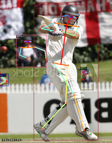
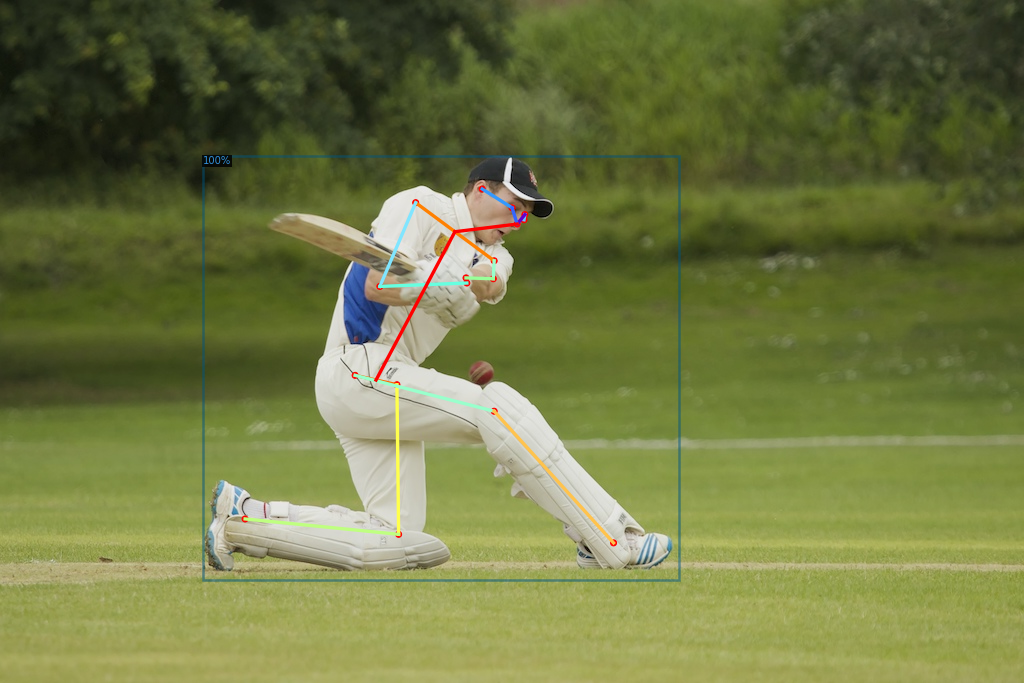
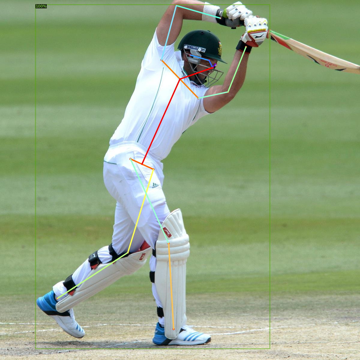
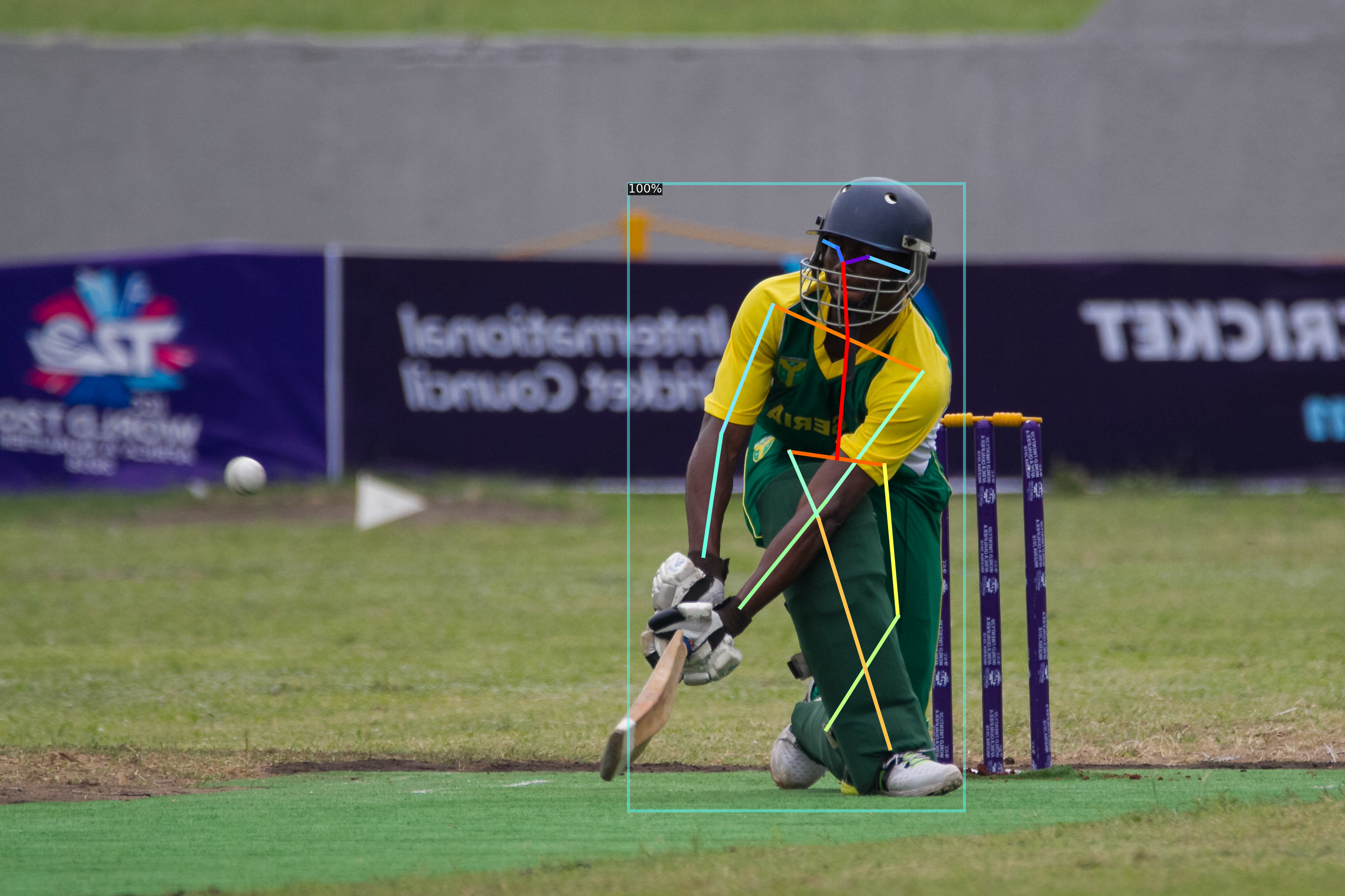
Let’s visualize a few predictions from the model. Here we are randomly picking five images and then for each image, we are taking the predictions defining the visualizer and drawing the predictions on the image, and finally plotting the predictions.
# for drawing predictions on images
from detectron2.utils.visualizer import Visualizer
# to obtain metadata
from detectron2.data import MetadataCatalog
# to display an image
from google.colab.patches import cv2_imshow
# randomly select images
for img in random.sample(images,5):
    # make predictions
    outputs = predictor(img)
    # use `Visualizer` to draw the predictions on the image.
    v = Visualizer(img[:, :, ::-1], MetadataCatalog.get(cfg.DATASETS.TRAIN[0]), scale=1)
    # draw prediction on image
    v = v.draw_instance_predictions(outputs["instances"].to("cpu"))
    # display image
    cv2_imshow(v.get_image()[:, :, ::-1])
Source:- Author
So here are the predictions from the model. You can see that we have bounding boxes along with the key points predicted for each of these players. You can see that the model has even predicted some of the images in the background as well. So these are a few predictions from the model.
Next, we are going to define a function that will be used to extract and detect the poses for the images. So this function will take an image as input make these predictions for the image using the pre-trained model and then convert the extracted key points into a numpy array for a single image.
There can be multiple objects as well. So we will select the object which has the highest score and keep only those key points and then finally we are converting the key points to a 1d array.
Since we wish to build a neural network model on top of that and the neural network takes a single-dimensional input.
So here we are converting it into a single dimension now we are going to use the defined function and extract the key points for all the images and store them in a list key point.
Now we have the key points for all the images. Next, we are going to build a neural network that will classify these key points into the type of shots.
# define function that extracts the keypoints for an image
def extract_keypoints(img):
  # make predictions
  outputs = predictor(img)
  # fetch keypoints
  keypoints = outputs['instances'].pred_keypoints
  # convert to numpy array
  kp = keypoints.cpu().numpy()
  # if keypoints detected
  if(len(keypoints)>0):
    # fetch keypoints of a person with maximum confidence score
    kp = kp[0]
    kp = np.delete(kp,2,1)
    # convert 2D array to 1D array
    kp = kp.flatten()
    # return keypoints
    return kp
# progress bar
from tqdm import tqdm
import numpy as np
# create list
keypoints   = []
# for every image
for i in tqdm(range(len(images))):
  # extract keypoints
  kp = extract_keypoints(images[i])
  # append keypoints
  keypoints.append(kp)
5. Classifying cricket shot using pose of a player
First of all, we are going to normalize the values of our key points which will eventually speed up the training process.
# for normalization
from sklearn.preprocessing import StandardScaler
# define normalizer
scaler= StandardScaler()
# normalize keypoints
keypoints = scaler.fit_transform(keypoints)
# convert to an array
keypoints = np.array(keypoints)
So here we have normalized the values of our key points. We are converting our target which is currently in the text form into numbers using the label encoding.
# converting the target categories into numbers
from sklearn.preprocessing import LabelEncoder
le = LabelEncoder()
y=le.fit_transform(labels)
After that, we are splitting our dataset into the training and the validation sets using the train test split function. So we have kept the test size as 0.2 which means 80(%) of the data will be used for training and 20(%) will be in the validation set.
# for creating training and validation sets
from sklearn.model_selection import train_test_split
# split keypoints and labels in 80:20
x_tr, x_val, y_tr, y_val = train_test_split(keypoints, y, test_size=0.2, stratify=labels,
                                        random_state=120)
Now in order to use the key points and the targets, we must convert them into tensors. Hence here we are converting the key points as well as the targets into python tensors for both the training and the validation set.
# converting the keypoints and target value to tensor
import torch
x_tr = torch.Tensor(x_tr)
x_val = torch.Tensor(x_val)
y_tr = torch.Tensor(y_tr)
y_tr = y_tr.type(torch.long)
y_val = torch.Tensor(y_val)
y_val = y_val.type(torch.long)
Here is the shape of the training and the validation set has 464 images for training and 116 for validation.
# shape of training and validation set
(x_tr.shape, y_tr.shape), (x_val.shape, y_val.shape)
Now we will define the architecture for our model. So here we are importing a few functions from PyTorch that will help us. Here we are defining a simple neural network architecture with just one hidden layer with 64 neurons.
The output layer has four neurons since we have four different classes and the activation function of the output layer will return probabilities. Hence we have a softmax activation function.
# importing libraries for defining the architecture of model
from torch.autograd import Variable
from torch.optim import Adam
from torch.nn import Linear, ReLU, Sequential, Softmax, CrossEntropyLoss
# defining the model architecture
model = Sequential(Linear(34, 64),
                   ReLU(),
                   Linear(64, 4),
                   Softmax()
                   )
Next, we are defining the optimizer as adam and the loss as cross-entropy. It is a multi-class classification problem and then we are transferring the model to GPU.
# define optimizer and loss function
optimizer = Adam(model.parameters(), lr=0.01)
criterion = CrossEntropyLoss()
# checking if GPU is available
if torch.cuda.is_available():
    model = model.cuda()
    criterion = criterion.cuda()
Next, we are defining a function that will be used to train our model. So this function will take the number of epochs as input. We are going to set the model to train. Firstly we are initializing the loss as zero then we are loading the training and the validation set using the Pytorch variable.
Transferring our model and validation to GPU after that we are clearing the gradients of the model parameter. Next, we are taking the predictions from the model for both the training as well as the validation sets and sorting them into separate variables.
We have calculated the train and validation loss and finally, we are back-propagating the gradients and updating the parameters.
Additionally, we are also printing the validation loss after every 10th epoch.
def train(epoch):
    model.train()
    tr_loss = 0
    # getting the training set
    x_train, y_train = Variable(x_tr), Variable(y_tr)
    # getting the validation set
    x_valid, y_valid = Variable(x_val), Variable(y_val)
    # converting the data into GPU format
    if torch.cuda.is_available():
        x_train = x_train.cuda()
        y_train = y_train.cuda()
        x_valid = x_valid.cuda()
        y_valid = y_valid.cuda()
    # clearing the Gradients of the model parameters
    optimizer.zero_grad()
    # prediction for training and validation set
    output_train = model(x_train)
    output_val = model(x_valid)
    # computing the training and validation loss
    loss_train = criterion(output_train, y_train)
    loss_val = criterion(output_val, y_valid)
    # computing the updated weights of all the model parameters
    loss_train.backward()
    optimizer.step()
    if epoch%10 == 0:
        # printing the validation loss
        print('Epoch : ',epoch+1, 't', 'loss :', loss_val.item())
Now we have defined our function. We will use this train function and start the training for our model. Also, we are training 400 epochs. You can see that the model is printing loss at every 10th epoch.
Finally, we started with a loss of 1.38 and now we have a loss of 0.97 at the end. So we can see that the model performance is improving as the model training progresses.
# defining the number of epochs
n_epochs = 100
# training the model
for epoch in range(n_epochs):
    train(epoch)
Evaluating model performance
Let’s evaluate the model performance so we are going to check the accuracy of the model.
Hence importing the function from sklearn. we are getting the validation set including the key points as well as the target variables. Once you get the variable first transfer these values to GPU that we are taking the predictions from the model on the validation images using the trained model.
Now we are converting the predicted probabilities to the respective classes using the arg max function.
# to check the model performance
from sklearn.metrics import accuracy_score
# get validation accuracy
x, y = Variable(x_val), Variable(y_val)
if torch.cuda.is_available():
  x_val = x.cuda()
  y_val = y.cuda()
pred = model(x_val)
final_pred = np.argmax(pred.cpu().data.numpy(), axis=1)
accuracy_score(y_val.cpu(), final_pred)
Finally, we calculated the accuracy score so the accuracy of this model comes out to be 0.79 which is approximately 80 %.
Conclusion
In order to improve the accuracy, you can play around with different hyperparameters like increasing the number of hidden layers in the model, changing the optimizer, changing the activation function, increasing the number of epochs, and much more.
I hope you are already familiar with the hyperparameter tuning for the neural networks do try them out at your end and share your performance in the comment section. So this is how we can build a model to classify the shots using the pose of a player.
About the Author
Hi, I am Kajal Kumari. have completed my Master’s from IIT(ISM) Dhanbad in Computer Science & Engineering. As of now, I am working as Machine Learning Engineer in Hyderabad. Here is my Linkedin profile if you want to connect with me.
End Notes
Thanks for reading!
I hope that you have enjoyed the article. If you like it, share it with your friends also. Please feel free to comment if you have any thoughts that can improve my article writing.
If you want to read my previous blogs, you can read Previous Data Science Blog posts from here.
The media shown in this article is not owned by Analytics Vidhya and are used at the Author’s discretion.


%202.jpg)