This article was published as a part of the Data Science Blogathon.
Till now we have covered different pre-trained models for the image-classification tasks and we have a fair understanding of object detection, and we looked at the different architectures that can be used for solving the object detection problems.
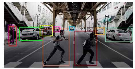
To summarize object detection involves identifying objects along with their locations. In this article, we’ll understand one of the use cases of object detection, which is face detection.
Table of Contents
1. Introduction to Face Detection
2. Application of Face Detection
3. Understanding the Problem Statement: WIDER FACE
4. Converting the annotations of the WIDER FACE dataset as per Detectron2
5. Steps to solve the Face Detection problems
Let’s start…….
Introduction to Face Detection
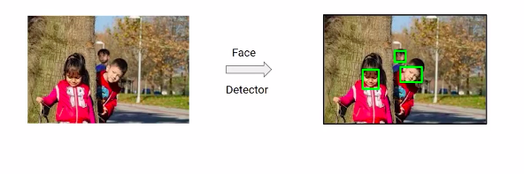
Similar to object detection, in face detection problems, the purpose is to identify faces from the image, along with their locations.
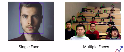
And we can see in the above images that we can have a single face in an image and multiple faces. In this article, we’ll learn both of these tasks. That is, how to detect faces when there is a single face in the image and the same for multiple phases in the image.
So by the end of this article, you’ll be able to build models that can detect either a single face or multiple faces from the image.
Let’s first look at some interesting applications of face detection.
Application of Face Detection
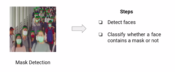
Face detection can be used to check if a person is wearing a mask or not. The steps for building such a model would be to detect the faces from the image first and then predict if the faces contain a mask or not.
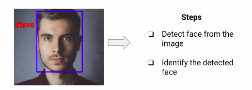
This is just one of the use cases of face detection. Face Recognition can be another use case. Here, we have to identify the person present in the image. So, to solve this problem, we’ll first have to detect the faces from the image and then identify the faces.
There can be multiple other applications, like installing CCTV cameras that can identify persons to prevent ATM machine robberies or to build a user-friendly check-in system at the airports.

These are some of the use cases, and applications of face detection, which we have mentioned in this section. Can you think of other applications of face detections? Feel free to share your thoughts in the comment section. In the next section, we’ll understand the problem statement that we have picked for face detection.
Understanding the Problem Statement: WIDER FACE
So in this section, we’ll understand the problem statement that we have picked for this article.
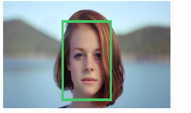
The objective of this article is to build a model that can detect faces from the images. So by the end of this article, we’ll be able to build a model that can take images as shown here. As an input, detect the faces in that image that returns the bounding boxes for the locations of these faces present in the image.
So we’ll be training the model, and we know that in order to train the model, we need the training data. So let’s look at the dataset that we’ll be using in order to train the face detection model.
In this module, we’ll be using the wider face dataset, which is benchmark data for the face detection tasks. It contains more than 32000 images comprising of approximately 0.4 million faces and this data set contains images and faces which have a large variation in scale, occlusion pose and so on.
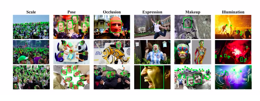
So scale basically refers to the image size, and based on the size of the image, the dataset is grouped into three scales: small, medium and large.
Similarly, occlusion also has three categories, which is no occlusion, partial occlusion and heavy occlusion. The wider dataset contains images from a range of 60 even categories like the parade, festival, football, tennis and many more.
So the diversity of the data set is huge, and these even categories are further divided into three sets based on the ease of detection which is easy, medium and hard.
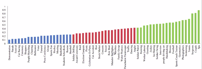
The categories marked in the above image, green belong to the easy set, those in red belong to the medium Set, and the blue ones belong to the hard Set. In this article, we’ll be working with images belonging to the easy Set.
Also, we’ll be using the detectoron2 library in order to build the face detection model, since it provides the state-of-the-art implementation for object detection tasks.
And by now, we know that in order to work with detectron2, our dataset must follow a specific format. So in the next section, we’ll first look at the format of the wider phase data set and then see how the dataset should be pre-processed in order to use it for the directron2 library.
Converting the Annotations of the WIDER FACE Dataset as per Detectron2
Till now we have understood the face detection problem and the dataset which we’ll be using to build the face detection model. In the above section, we discussed that we’ll be using detectron2 to build the model.
So, let’s quickly have an overview of detectron2. detectoron2 is a platform for object detection and segmentation tasks. It is created by the research team of Facebook AI. And detectron2 implements state-of-the-art architectures like faster R-CNN retina net and so on.
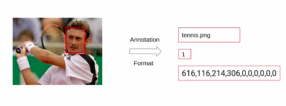
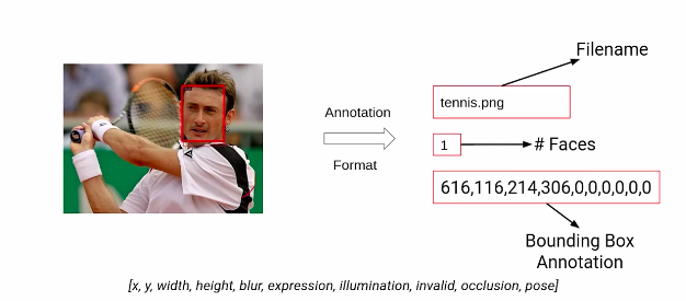
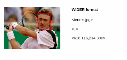
Now, let’s look at the format of the dataset we currently have. So, this is what the annotations of the wider face dataset look like. We have images containing faces, and corresponding to these images, we have the annotations.
The first thing here represents the file name then we have the number of faces present in a particular image. And since this image has a single face the value here is one. Finally, we have the bounding box coordinates for this image. These bounding boxes follow the following format. We have the x-min,y-min values followed by the height and width of the bounding box. Also, We have the values representing the different measures of variabilities that we have discussed in the above section, Including the blur expression, illumination, occlusion and so on.
So this is what the annotations of wider face data sets look like. Now here is another example from the dataset.
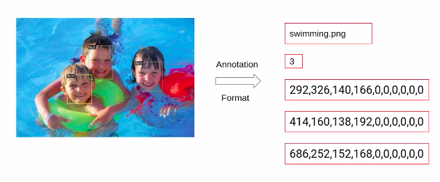
So first of all we have the image name, followed by the number of faces in the image that is 3 in this case, followed by the bounding box coordinates. The bounding boxes for each face are represented using a separate dictionary. For this image, since we have three faces, there will be three different dictionaries.
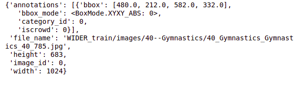
Now, the above image is the annotation from the wider phase dataset. And in order to use this dataset in detectron2, we must convert the annotations to this format as shown below.
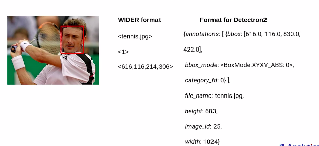
So, we first have a dictionary for the bounding boxes. and instead of having x-min, y-min, width and height for detectron2. We should have the x-min, y-min, x-max and y-max values that we’ll be using here. The category id here represents the category of this image. Then we have to pass the file name, which will be the name of the above image, followed by the height, width and image id.
So this is the format that detectron2 expects as input and hence we’ll have to pre-process our data accordingly. So while creating the face detection model we’ll be pre-processing these input formats into the format required for detectron2.
So that’s all on the data preparation part. in the next section, we’ll discuss the steps that we’ll be following to build the face detection model, and then finally we will work on the implementation.
Steps to Solve the Face Detection Problem
In this section, we will look at the steps that we’ll be following, while building the face detection model using detectron2. So we’ll start with these steps:-
- Install Dependencies
- Loading and pre-processing the data
- Creating annotations as per Detectron2
- Register the dataset
- Fine Tuning the model
- Evaluating model performance
I have already uploaded the dataset on the drive and in order to run the notebooks at your end, you should also upload the data set on your drive.
Dataset Link:- https://drive.google.com/drive/folders/1bbPG4pcMT_rMyqInAissTsIOMYJ3rnPj
So, here are the files which are available in the dataset. we have an easy.txt file, that includes the names of classes belonging to the easy set. Then we have the wider space split.zip which contains the annotations for images in the training and the validation set. WIDER_train contains the training images and WIDER_val contains the validation images.
Building a face detection model to detect single faces
Till now we have understood what is face detection, how we have to annotate the data set as per detectron2 and the steps that we’ll be following to build our face detection model.
Now as already discussed, there can be scenarios where we have only a single face in the image and there can be situations where the task is to detect multiple faces in the images.
So in this article, we’ll solve both of these tasks. We’ll first build a model that can detect a single face from the image, and then we’ll build another model which will be able to detect multiple objects from the image. So, in this article, our focus will be on building a model that can detect a single face. So to build a face detection system that can detect a single face from the image, a few steps that we are going to follow, which we have discussed in the last section.
1. Install Dependencies
We’ll first start with installing all the dependencies. First of all, we are installing the 5.1 version of the PYML library. This is a prerequisite for detectoron2. And if we have an older version of this library some of the functionalities of detectron2 might not work correctly.
Then we are installing the detectron2 library and we have seen this step earlier while we were implementing the RetinaNet model.
# install required version
!pip install pyyaml==5.1
# installing detectron2
!pip install detectron2==0.1.3 -f https://dl.fbaipublicfiles.com/detectron2/
                    wheels/cu101/torch1.5/index.html
2. Loading and pre-processing the data
The next step is to load the dataset and preprocess it. since the data set is present in google drive, we have to first mount the drive.
# mounting drive
from google.colab import drive
drive.mount('drive')
Next, we are extracting the files which are in the zip format. So we are extracting our training, validation, and annotations. Now we are reading the annotation files for both the training and the validation set.
# extracting files
!unzip '/content/drive/My Drive/Wider_dataset/WIDER_train.zip'
!unzip '/content/drive/My Drive/Wider_dataset/WIDER_val.zip'
!unzip '/content/drive/My Drive/Wider_dataset/wider_face_split.zip'
So to read the files, we’ll be using the pandas library and hence importing that here first. And then we are specifying the paths for the annotation files of the training and the validation set and then read them using the read_csv function of pandas.
# reading files
import pandas as pd

# specify path of the data
path_train = '/content/wider_face_split/wider_face_train_bbx_gt.txt'
path_val = '/content/wider_face_split/wider_face_val_bbx_gt.txt'

# reading data
train = pd.read_csv(path_train,header=None)
val = pd.read_csv(path_val,header=None)
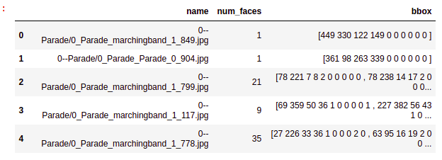
Let’s quickly look at the CSV files. So here are the first 10 rows from the train CSV file that we have. Here we have the file names followed by the number of faces in that image, and then the bounding box coordinates and the same part. And you can see is repeated. So currently the format is not readable. So let’s convert this format to a more meaningful and readable form. Which should look something like this. We would want the format where we have names in a separate column then numbers of faces as a separate variable and then the bounding box coordinates. hence we’ll reformat the data set accordingly.
# pre-processing data
# this function accepts the dataframe and returns modified dataframe
def reformat(df):
  # fetch values of first column
  values = df[0].values
  # creating empty lists
  names=[]
  num_faces=[]
  bbox=[]
  # fetch values into corresponding lists
  for i in range(len(values)):

      # if an image
      if ".jpg" in values[i]:

        # no. of faces
        num=int(values[i+1])

        # append image name to list
        names.append(values[i])

        # append no. of faces to list
        num_faces.append(num)

        # create bbox list
        box=[]
        for j in range(i+2,i+2+num):
          box.append(values[j])

        # append bbox list to list
        bbox.append(box)

  return pd.DataFrame({'name':names,'num_faces':num_faces,'bbox':bbox})
we are going to convert the training and the validation data sets and store it as train and val.
# pre-processing the data
train = reformat(train)
val = reformat(val)
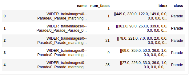
So let’s look at the first few rows of these data sets. So we are first printing the head of the train. you can see that this data set is now in the required format.
# first 5 rows of the pre-processed data
train.head()
let us also look at the shape of the training data and the shape of the validation data. so we can see that in the training data we have 12 880 rows and in the validation, we have 3226 rows.
# shape of the training data
train.shape
The output is:- (12880, 3)
# shape of validation data
val.shape
The output is:- (3226, 3)
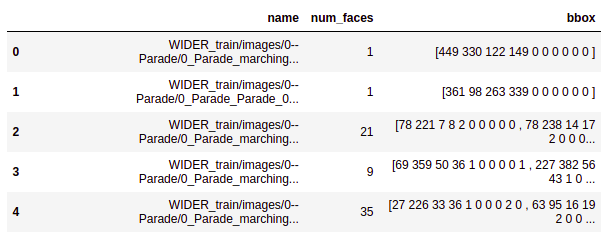
Next, we’ll do some pre-processing on this data set so here we are adding the complete path before the file name and for training, we are adding the path wider_ train/images and for validation, the path will be wider_val/images.
# adding full path
train['name'] = train['name'].apply(lambda x: 'WIDER_train/images/'+x )
val['name']   = val['name'].apply(lambda x: 'WIDER_val/images/'+x )
After applying this the new dataset would look something like the below image. So we’ll have the complete path for all of these images.
# first 5 rows
train.head()
Next, we are converting the bounding box coordinates to floating points using the float_function of the numpy library. Hence we are first importing the numpy library here and then converting the bounding box coordinates for both training and the validation set and again printing the first five rows of the data set.
# converting bbox to floating point
import numpy as np
train['bbox'] = train['bbox'].apply
                        (lambda row:[ np.float_(annos.split()) for annos in row] )
val['bbox']   = val['bbox'].apply
                    (lambda row:[ np.float_(annos.split()) for annos in row] )
# first 5 rows
train.head()
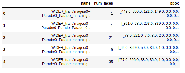
So the above image, the output confirms that the bounding boxes are converted into floating points. Here so you can see this is bbox column value 27.0, 26.0, and so on.
Next, we are going to extract the class names from the names of the images. So remember that we discussed previously will only be using the images belonging to the easy set. Hence these class names will help us to get the images which are belonging to the easy set. So here we are extracting the class name from the name of the images and
storing them in a new variable named as a class for both the training as
well as the validation data sets.
# extracting class names
train['class']= train['name'].apply(lambda x:x.split("/")[2].split("--")[1])
val['class']  = val['name'].apply(lambda x:x.split("/")[2].split("--")[1])
# first 5 rows
train.head()
you can see that now we have a new column class that has the class against each of these images.
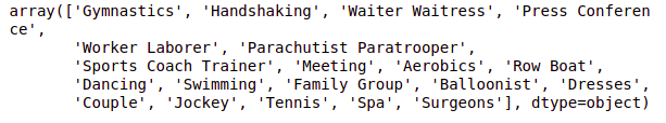
Next, we are going to read the easy.txt file which contains the names of the classes belonging to the easy set. So we are reading this file here using the read_csv function and printing the values that we get.
# reading class names
easy_df = pd.read_csv('drive/My Drive/Wider_dataset/easy.txt',header=None)
easy_labels = easy_df[0].values
# easy labels
easy_labels
Here is a list of the classes that belong to the easy set. so we have a total of 20 classes here.
Now we’ll select only those images which belong to any of these above-mentioned classes. So here we are running a for loop for only the easy classes and fetching the rows which have the easy categories.
# creating empty dataframes
train_df, val_df= pd.DataFrame(), pd.DataFrame()
# fetching rows of easy classes only
for i in easy_labels:
  train_df = pd.concat( [train_df, train[train['class']==i]] )
  val_df   = pd.concat( [val_df, val[val['class']==i]] )
We have taken a subset from the data set for both training and validations. As discussed earlier the aim of this article is to build a face detection model that will work for single faces and hence we are only selecting those images which have a single face so we are doing this for both our training and validation.
Now before we go ahead, let’s quickly check the train shape and the validation shape.
# shape of dataframe
train_df.shape, val_df.shape
So we have 1000 images in train and 274 images in the validation data. Next, We will see how to convert the annotations of a wider dataset to the annotations of Detectron2.
3. Creating annotations as per Detectron2
Now, we’ll convert the annotations of our dataset as per the requirements of the detectoron2 library. So here is what the annotations should look like. We’ll first have the file name and then the number of faces in that image followed by the bounding box coordinates which are of the format Xmin, Ymin, width, and height, and finally the class.
So we want the annotations to be in the below format. We’ll first see how to get this format for a single image and then we’ll write a generalized function that will convert the annotations format for all of these images.
# custom annotation format
idx=0
values = train_df.values[idx]
print(values)
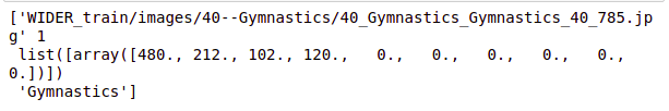
Source:- Author
# for dealing with images
import cv2
# create annotation dict
record = {}
# image name
filename = values[0]
# height and width of an image
height, width = cv2.imread(filename).shape[:2]
# creating fields
record["file_name"] = filename
record["image_id"] = 0
record["height"] = height
record["width"] = width
# different ways to represent bounding box
from detectron2.structures import BoxMode
# create bbox list
objs = []

# for every face in an image
for i in range(len(values[2])):

  # fetch bbox coordinates
  annos = values[2][i]
  # unpack values
  x1, y1, w, h = annos[0], annos[1], annos[2], annos[3]

  # find bottom right corner
  x2, y2 = x1 + w, y1 + h

  # create bbox dict
  obj = {       "bbox": [x1, y1, x2, y2],
                "bbox_mode": BoxMode.XYXY_ABS,
                "category_id": 0,
                "iscrowd": 0
        }
  # append bbox dict to bbox list
  objs.append(obj)
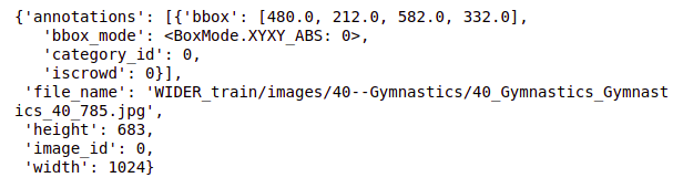
# assigning bbox list to annotation dict
record["annotations"] = objs
# standard annotation format
record
The output is:-
def create_annotation(df):

  # create list to store annotation dict
  dataset_dicts = []
  # for each image
  for idx, v in enumerate(df.values):

    # create annotation dict
    record = {}
    # image name
    filename = v[0]
    # height and width of an image
    height, width = cv2.imread(filename).shape[:2]
    # assign values to fields
    record["file_name"] = filename
    record["image_id"] = idx
    record["height"] = height
    record["width"] = width
    # create list for bbox
    objs = []
    for i in range(len(v[2])):
      # bounding box coordinates
      annos = v[2][i]

      # unpack values
      x1, y1, w, h = annos[0], annos[1], annos[2], annos[3]

      # find bottom right corner
      x2, y2 = x1 + w, y1 + h

      # create bbox dict
      obj = {   "bbox": [x1, y1, x2, y2],
                "bbox_mode": BoxMode.XYXY_ABS,
                "category_id": 0,
                "iscrowd": 0
            }
      # append bbox dict to a bbox list
      objs.append(obj)

    # assign bbox list to annotation dict
    record["annotations"] = objs
    # append annotation dict to list
    dataset_dicts.append(record)

  return dataset_dicts
# create standard annotations for training and validation datasets
train_annotation = create_annotation(train_df)
val_annotation = create_annotation(val_df)
# standard annotation of an image
train_annotation[0]
4. Register the dataset
To let detectron2 know how to obtain a dataset, we will implement a function that returns the items in your dataset and then tell detectron2 about this function. For this, we will follow these steps:
1. Register your dataset (i.e., tell detectron2 how to obtain your dataset).
2. Optionally, register metadata for your dataset.
We are going to register it on detectron2. So we are first importing the required functions from detectron2.data which are dataset catalog and meta catalog. We are registering the data and naming it as face_train.
from detectron2.data import DatasetCatalog, MetadataCatalog
# register dataset
DatasetCatalog.register("face_train", lambda d="train": create_annotation(train_df))
We are also registering the metadata where we are defining the class as a face since we want to detect faces.
# register metadata
MetadataCatalog.get("face_train").set(thing_classes=["face"])
Next, let us visualize a few samples from the training set. So for that, we are first importing the visualizer function from detectoron2 and cv2_imshow. In order to visualize the images, we are going to import random. Since we are going to randomly pick the images. So here we are getting the names of the classes from the metadata catalog and we are printing the names.
# for drawing bounding boxes on images
from detectron2.utils.visualizer import Visualizer
# for displaying an image
from google.colab.patches import cv2_imshow
# for randomly selecting images
import random
# get the name of the classes
face_metadata = MetadataCatalog.get("face_train")
print(face_metadata)
So we are randomly picking five images from the training set and this is done using “random.sample” then we are reading the images using cv2.imread and using the visualizer function. We are going to visualize the bounding boxes using draw_dataset_dict. And also We are plotting the bounding boxes for the faces and finally using “cv2_imshow“. Now we are going to print the image along with these bounding boxes.
# randomly select images
for d in random.sample(train_annotation, 5):

  # read an image
  img = cv2.imread(d["file_name"])
  # create visualizer
  visualizer = Visualizer(img[:, :, ::-1], metadata=face_metadata, scale=0.5)

  # draw bounding box on image
  vis = visualizer.draw_dataset_dict(d)

  # display an image
  cv2_imshow(vis.get_image()[:, :, ::-1]
Till now the data preparation part is done in the next section we’ll train our face detection model.
5. Fine-Tuning the model
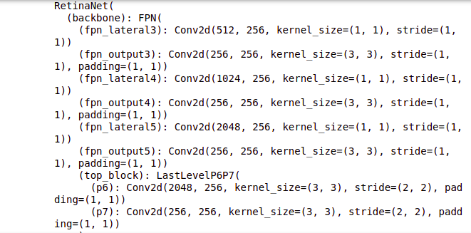
Now our dataset is ready. Let’s train the model. We will take a pre-trained model and fine-tune it as per our problem. So we’ll be using the retina net pre-trained model which is trained on the coco data set. Since our wider face data set is different from the coco data set will retrain the entire architecture of the pre-trained model as per our problem.
So here we are first importing a few helper functions which are model_zoo.
In order to load the pre-trained model default trainer will be used to train the model and get_cfg which will be used to get the configurations of the pre-trained model.
Next, we are defining the configuration instance and first of all, we are specifying the path of the pre-trained model in this configuration file, and then we are loading the weight of the “retainnet ” pre-trained model which is trained on the coco detection data set.
# to obtain pretrained models
from detectron2 import model_zoo
# to train the model
from detectron2.engine import DefaultTrainer
# set up the config
from detectron2.config import get_cfg
# interact with os
import os
# define configure instance
cfg = get_cfg()
# Get a model specified by relative path under Detectron2’s official configs/ directory.
cfg.merge_from_file(model_zoo.get_config_file("COCO-Detection/retinanet_R_50_FPN_1x.yaml"))
# load pretrained weights
cfg.MODEL.WEIGHTS = model_zoo.get_checkpoint_url("COCO-Detection/retinanet_R_50_FPN_1x.yaml")
Next, we have to define the name of the train and the test data set in the configuration file and these data sets must be registered in “detectron 2”. We have registered the training data set as face_train and hence we are giving the name here. Currently, we do not want any test data and hence we are keeping this blank.
# List of the dataset names for training. Must be registered in DatasetCatalog
cfg.DATASETS.TRAIN = ("face_train",)
cfg.DATASETS.TEST = ()
Now, we are defining a few hyperparameters for our model. Our model is defined, and we have changed the hyperparameters, it’s time to train the model.
# no. of images per batch
cfg.SOLVER.IMS_PER_BATCH = 2
# set base learning rate
cfg.SOLVER.BASE_LR = 0.001
# no. of iterations
cfg.SOLVER.MAX_ITER = 1000
# only has one class (face)
cfg.MODEL.ROI_HEADS.NUM_CLASSES = 1
So we are creating a directory, which will save the weights for the model, as the training progresses. Exist_score will tell us if the directory already exists or not. Setting this as true will mean that the directory already exists.
Now, using the modified configuration file we are creating a trainer using the default_trainer function, and using resume or load, we can set if we want to start the training from scratch, or resume using the pre-trained weights.
If the resume is set to true, and the last checkpoint exists, it will load the checkpoints, and start training on top of that.
If this is set to false, which is in our case, the training will start from the first iteration. So since we are training the model from the first iteration, we are going to set this resume is equal to false.
The summary of the model will be printed after every iteration, which will include the total loss, the classification loss, regression loss, the time taken to train for a few iterations, the learning rate after that particular iteration, and the maximum memory used.
# create directory to save weights
os.makedirs(cfg.OUTPUT_DIR, exist_ok=True)
# create a trainer with given config
trainer = DefaultTrainer(cfg)
# If resume==True, and last checkpoint exists, resume from it, load all checkpointables (eg. optimizer and scheduler) and update iteration counter.
# Otherwise, load the model specified by the config (skip all checkpointables) and start from the first iteration.
trainer.resume_or_load(resume=False)
# train the model
trainer.train()
The output of this training model is:-
Source:- Author
All right we can see that now the training is complete, as the training progresses, we can see that the loss keeps decreasing, for every subsequent iteration. If you observe both the classification loss and the regression loss, you will see a decreasing trend here.
To visualize the results of this training more efficiently, and in a better way, we’ll use the tensorboard. Tensorboard provides visualization needed for machine learning and deep learning. We can track and visualize the metrics like loss and accuracy. We can also visualize the parameters learned by the model and so on so.
# Look at training curves in tensorboard:
%load_ext tensorboard
%tensorboard --logdir output
We are going to use this visualization tool in order to visualize the training of our model.
So let us first visualize the total loss, and here we can see that we have plots for the regression loss and the classification loss. We can see that both for regression as well as for classification the loss keeps decreasing with the increasing number of iterations.
And if we check the plot for the learning rate and how it changes with the number of iterations, we can see that the learning rate keeps increasing with the increasing number of iterations. Similarly, we can visualize other factors as well.
6. Evaluating model performance
Finally, we’ll evaluate the performance of this model on the validation set. And in order to use any data set in detectron2, we must register it first. So we are going to register the validation data set similar to how we register the training data set.
we are going to name this as face_val we are also registering the metadata where we are defining the classes that are present in this data set which is the face.
# register validation dataset
DatasetCatalog.register("face_val", lambda d="val": create_annotation(val_df))
# register metadata
MetadataCatalog.get("face_val").set(thing_classes=["face"])
Next, we are loading the weights of the model which were saved as “model _final.pth” during the training. And we are keeping the score threshold as 0.8.
# load the final weights
cfg.MODEL.WEIGHTS = os.path.join(cfg.OUTPUT_DIR, "model_final.pth")
# set the testing threshold for this model
cfg.MODEL.RETINANET.SCORE_THRESH_TEST = 0.8
# List of the dataset names for validation. Must be registered in DatasetCatalog
cfg.DATASETS.TEST = ("face_val", )
We are also specifying the test set in the configuration file.
After this, we are defining the predictor function using the default
predictor and pass the updated configuration file inside it.
# set up predictor
from detectron2.engine import DefaultPredictor
# Create a simple end-to-end predictor with the given config that runs on single device for a single input image.
predictor = DefaultPredictor(cfg)
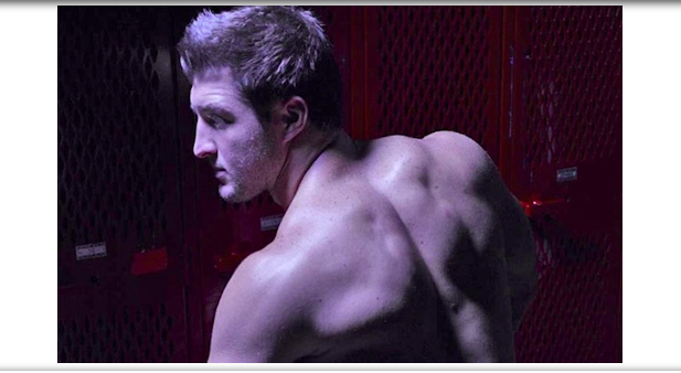
Let us now visualize the predictions on a few of the images, from the validation set. So we are going to randomly pick the images from the validation set, and here we are randomly picking three images. We are reading these images and taking the predictions from the predictor function, then creating the visualizations for these images.
So we are drawing the bounding boxes and printing these bounding boxes over the images and plotting the output using the cv2_imshow function. So here you can see that on this image the face is clearly detected with 95 % accuracy.
# create standard annotations for validation data
dataset_dicts = create_annotation(val_df)
# randomly select images
for d in random.sample(dataset_dicts,3):

    # read an image
    im = cv2.imread(d["file_name"])

    # make predictions
    outputs = predictor(im)

    # create visualizer
    v = Visualizer(im[:, :, ::-1], metadata=face_metadata, scale=0.5)

    # draw predictions on the image
    v = v.draw_instance_predictions(outputs["instances"].to("cpu"))

    # display image
    cv2_imshow(v.get_image()[:, :, ::-1])
Similarly on this image also we have the face detected with 98 %probability.
Source:- Author
let us now check the performance on the entire validation set. So for that, we are importing the coco evaluator and inference on the data set. These two functions are present within the detectorn2 evaluation module. In order to load the images from the validation set, we are going to use the build_detection_test_loader and we have imported that here as well.
So here we are using the coco evaluator that we imported, and creating the evaluators.
To this function we have to pass the validation data, the cfg file, and using this, the coco evaluator will be able to evaluate the performance on this validation set.
So val_loader is the loader for the validation set and the evaluator is used to evaluate the validation set. So here we have given in our val_loader and evaluator, to the function inference on the data set.
from detectron2.evaluation import COCOEvaluator, inference_on_dataset
from detectron2.data import build_detection_test_loader
# create a evaluator using COCO metrics
evaluator = COCOEvaluator("face_val", cfg, False, output_dir="./output/")
# create a loader for test data
val_loader = build_detection_test_loader(cfg, "face_val")
# runs the model on each image in the test data and produces the results
inference_on_dataset(trainer.model, val_loader, evaluator)
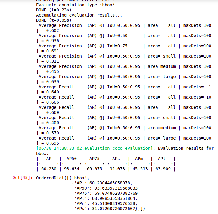
Source:- Author
So we have the results here it will print the total inference time taken, and then the model performance. So we got an average precision value of approximately 93 %, for an iou of 0.5 and for iou of 0.75.
We have approximately 70%. So this is how we can build a face detection model that can detect single faces from the images.
Conclusion
In this article, we solved the problem of detecting a single face in the image. Fundamentals of face detection are critical for solving the business challenge and developing the necessary model. When it comes to working with image data, the most difficult task is figuring out how to detect faces from images that can be applied to the model. While working on image data you have to analyze a few tasks such as face detection, bounding box.
I hope the articles helped you understand how to deal with image data, how to detect faces from images, we are going to use this technique, and apply it in a few domains such as the medical, sports analysis domain.
In real-life scenarios, there can be situations when we have multiple faces in a single image so in the next article let us will work on building a model that can detect multiple faces from the images. Hope you enjoyed reading this article on the To Build Face detection Systems.
Thank you.
About the Author
Hi, I am Kajal Kumari. have completed my Master’s from IIT(ISM) Dhanbad in Computer Science & Engineering. As of now, I am working as Machine Learning Engineer in Hyderabad. Here is my Linkedin profile if you want to connect with me.
End Notes
Thanks for reading!
I hope that you have enjoyed the article. If you like it, share it with your friends also. Please feel free to comment if you have any thoughts that can improve my article writing.
If you want to read my previous blogs, you can read Previous Data Science Blog posts from here.
The media shown in this article is not owned by Analytics Vidhya and are used at the Author’s discretion.
Kajal Kumari
07 Apr, 2022


