The Scientific Discipline of Computer Vision
This article was published as a part of the Data Science Blogathon.
Introduction
AI and machine vision, which were formerly considered futuristic technology, has now become mainstream, with a wide range of applications ranging from automated robot assembly to automatic vehicle guiding, analysis of remotely sensed images, and automated visual inspection. Computer vision and deep learning are two of the hottest topics these days, with every tech business and even start-up racing to stay ahead of the pack. In this article, We’ll look at some of the key ideas in Deep Learning for Computer Vision.
The scientific discipline of computer vision (CV) outlines how machines perceive the meaning of images and movies. Computer vision algorithms examine specific criteria in photos and videos and then apply interpretations to tasks that need prediction or decision-making.

Deep learning algorithms are now the most widely utilized in computer vision. This article examines the various applications of deep learning in computer vision. You’ll learn about the benefits of employing convolutional neural networks (CNNs), which have a multi-layered design that allows neural networks to focus on the most important aspects of a picture.
In computer vision, natural language processing, and video/speech recognition, deep learning has proved overwhelmingly effective. Computer Vision models can be used to perform tasks such as facial recognition, dog breed identification, and even tumor detection from CT scans: the possibilities are unlimited.
What is Computer Vision (CV)?
Computer vision is a subset of artificial intelligence (AI) that allows computers and systems to extract useful information from digital images, videos, and other visual inputs. In the same way that artificial intelligence allows computers to think, computer vision allows them to see, watch, and comprehend.
Human vision and computer vision are identical, with the exception that humans have an edge. Context has taught human eyesight how to identify objects distinctly, how far away they are, whether they are moving, and whether there is something wrong with a picture during the course of their lives.
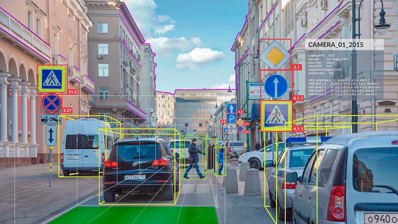
Computer vision trains computers to perform equivalent tasks in a fraction of the time by employing cameras, data, and algorithms instead of human retinas, optic nerves, and the visual brain. Because a system trained to check items or monitor a manufacturing asset can examine hundreds of products or processes per minute, it can quickly outperform people in detecting faults or concerns that would otherwise go undetected.
Image processing and computer vision are not the same things, even though they both deal with visual data. Modifying or altering images to generate a new result is what image processing entails. It can include brightening or darkening the image, boosting the resolution, obscuring sensitive data, or cropping. The distinction between image processing and computer vision is that the former does not always necessitate content recognition.
CNN: The Foundation of Modern Computer Vision
Convolutional neural networks (CNNs) are used in modern computer vision techniques, and they provide a significant performance boost over classic image processing algorithms.
CNNs are multi-layered neural networks that are used to reduce input and calculations to the most relevant set over time. The data entered is then compared to known data in order to identify or classify it. CNNs are commonly employed for computer vision applications, but they may also be utilized for text and audio analytics.
Each base colour utilized in the image (e.g. red, green, blue) is represented as a matrix of values when it is processed by a CNN. In the case of colour images, these values are evaluated and condensed into 3D tensors, which are collections of stacks of feature maps related to a region of the image.
The image is processed through a succession of convolutional and pooling layers, which take the most important data from each image segment and condense it into a smaller, representative matrix. This method is performed numerous times. The convolutional process’s final features are delivered to a fully connected layer, which generates predictions.
Deep Learning Architectures for Computer Vision
The architecture of a CNN determines its performance and efficiency. This comprises the structure of layers, the design of elements, and the elements that are present in each layer. Many CNNs have been developed, but the ones listed below are among the most effective.
AlexNet (2012)
The AlexNet architecture is based on the LeNet design. It has three fully linked layers and five convolutional layers. To facilitate the utilization of two GPUs during training, AlexNet has a dual pipeline layout.
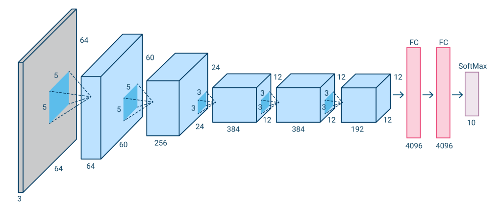
Instead of the sigmoid or Tanh activation functions used in typical neural networks, AlexNet uses rectified linear units (ReLU). AlexNet can train models faster because ReLU is simpler and faster to compute.
GoogleNet (2014)
The LeNet design underpins GoogleNet, also known as Inception V1. It consists of 22 layers made up of inception modules, which are small groupings of convolutions.
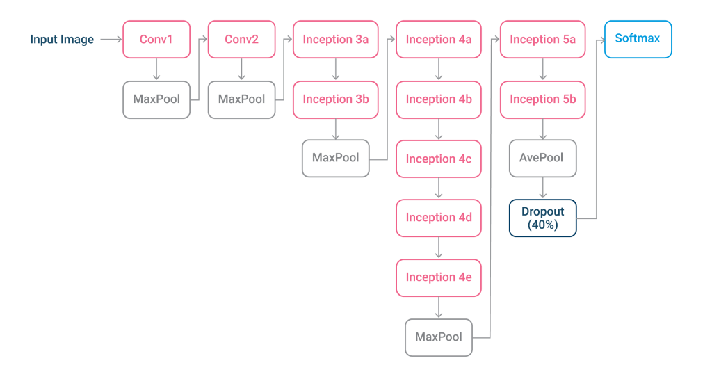
To decrease the number of parameters GoogleNet must process, these inception modules use batch normalization and RMSprop. RMSprop is a learning rate optimization approach that employs adaptive learning rate methodologies.
VGGNet (2014)
The VGG 16 architecture has 16 layers (some variants had 19 layers). VGGNet has convolutional layers, a pooling layer, a few more convolutional layers, a pooling layer, a few more convolutional layers, a pooling layer, and so on.

VGG is built on the idea of a much deeper network with smaller filters, it employs 3 convolutions throughout, which is the smallest convolution filter size that only looks at some of the neighboring pixels. Because there are fewer parameters, it uses modest filters, allowing for the addition of more layers. It has the same effective receptive field as one convolutional layer with seven layers.
Xception (2016)
Xception is an Inception-based architecture that uses depthwise separable convolutions to replace the Inception modules (depthwise convolution followed by pointwise convolutions).
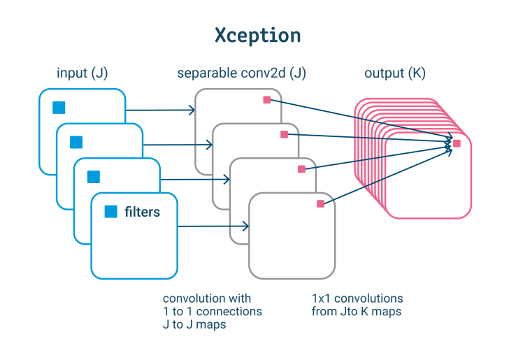
Xception captures cross-feature map correlations first, followed by spatial correlations. This makes it possible to make better use of model parameters.
The Promise of Deep Learning for Computer Vision
For computer vision, deep learning approaches are popular because they deliver on their promises. The three key promises of deep learning for CV are as follows:

- The Promise of Feature Learning: Instead of requiring feature detectors to be constructed and specified by an expert, deep learning approaches may automatically learn the features from picture data required by the model.
- The Promise of Continued Improvement: Deep learning’s performance in computer vision is based on real-world data, and the advances appear to be continuing, if not speeding up.
- The Promise of End-to-End Models: Massive end-to-end deep learning models can be fitted on large datasets of images or video, resulting in a more general and effective method.
Deep learning is required to reach the state-of-the-art on many tough problems in the field of computer vision, which has yet to be addressed.
Uses of Deep Learning in Computer Vision
Deep learning methods have made it possible to create more accurate and complicated computer vision models. The use of computer vision applications is becoming more valuable as these technologies advance. A few examples of how deep learning is being used to improve computer vision are listed below.

- Localization and object detection: The term “image localization” refers to the process of determining where items in an image are located. Objects are indicated with a bounding box once they have been identified. Object detection takes this a step further by classifying the objects that have been identified. CNNs are used in this technique.
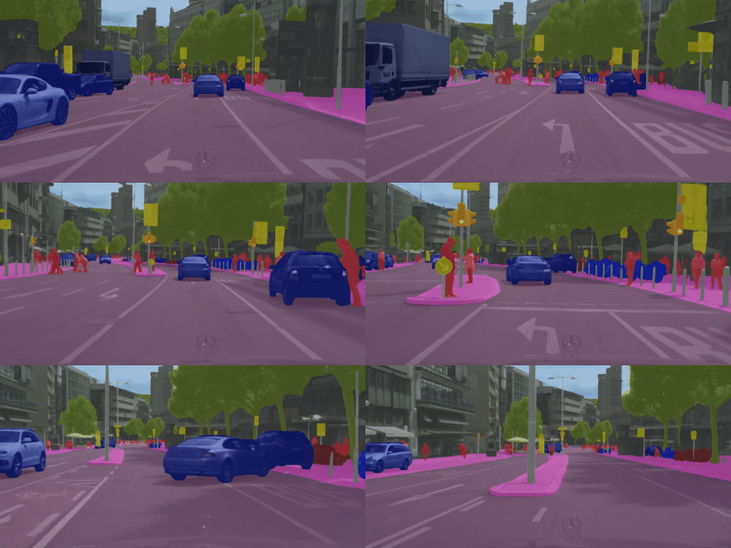
- Semantic segmentation: Object segmentation, also known as semantic segmentation, is similar to object detection except that it is based on the specific pixels that are associated with an object. This allows for a more precise definition of image objects without the need for bounding boxes. Fully convolutional networks (FCN) or U-Nets are frequently used for semantic segmentation. The training of autonomous vehicles is one notable use for semantic segmentation.
- Pose estimation: Pose estimate is a technique for determining where joints are in a photograph of a person or an item, as well as what their positioning signifies. Both 2D and 3D photos can be used with it. PostNet, a CNN-based architecture, is the most commonly used architecture for pose estimation. Pose estimation is a technique for predicting where portions of the body will appear in an image and can be used to create realistic human stances and motion.
Basic Python Implementation
Image Classification Model
A new standard dataset for computer vision and deep learning is the Fashion-MNIST clothes classification challenge. It’s a collection of 60,000 little square 2828 pixel grayscale photos of goods from ten different apparel categories, including shoes, t-shirts, dresses, and more.
The following example loads the dataset, scales the pixel values, then fits a convolutional neural network to the training dataset and assesses the network’s performance on the test dataset. On a modern CPU, the example will execute in a matter of minutes; no GPU is necessary.
from keras.datasets import fashion_mnist
from keras.utils import to_categorical
from keras.models import Sequential
from keras.layers import Conv2D
from keras.layers import MaxPooling2D
from keras.layers import Dense
from keras.layers import Flatten
# load dataset
(trainX, trainY), (testX, testY) = fashion_mnist.load_data()
trainX = trainX.reshape((trainX.shape[0], 28, 28, 1))
testX = testX.reshape((testX.shape[0], 28, 28, 1))
# convert from integers to floats
trainX, testX = trainX.astype('float32'), testX.astype('float32')
# normalize to range 0-1
trainX,testX = trainX / 255, testX / 255
# one hot encode target values
trainY, testY = to_categorical(trainY), to_categorical(testY)
# define model
model = Sequential()
model.add(Conv2D(32.0, (3.0, 3.0), activation='relu', kernel_initializer='he_uniform', input_shape=(28.0, 28.0, 1.0)))
model.add(MaxPooling2D())
model.add(Flatten())
model.add(Dense(100, activation='relu', kernel_initializer='he_uniform'))
model.add(Dense(10, activation='softmax'))
model.compile(optimizer='adam', loss='categorical_crossentropy', metrics=['accuracy'])
# fit model
model.fit(trainX, trainY, epochs=10, batch_size=32, verbose=2)
# evaluate model
loss, acc = model.evaluate(testX, testY, verbose=0)
print(loss, acc)
|
Conclusion
- Computer vision necessitates a large amount of data. It goes through the data processing process again and again until it identifies distinctions and, finally, recognizes images.
- Deep learning, a sort of machine learning, and a convolutional neural network (CNN) are two key technologies utilized in CV.
- Computer vision techniques are computationally expensive, and at scale, many GPUs may be required.
- Deep learning has revolutionized the field of computer vision, bringing effective answers to problems that had previously remained unsolvable.
The media shown in this article is not owned by Analytics Vidhya and are used at the Author’s discretion.


