A Comprehensive Guide on Deep learning for Computer vision

This article was published as a part of the Data Science Blogathon

Overview

1. Deep learning is the most powerful method used to work on vision-related tasks.
2. Convolutional Neural Networks or convents are a type of deep learning model which we use to approach computer vision-related applications.
3. In this guide, we will explore how CNN works and how they can be applied to an image classification task. We will also build a CNN model and train it on a training dataset from scratch using Keras.

Introduction

I have always been fascinated by the potential and power of deep learning models and how they can understand to perform tasks like Image classification, Image segmentation, Object detection, etc. We have also come across some segmentation algorithms like tumors/abnormalities detection from X-rays where they have outperformed doctors in the same.

In this guide, we will go through CNN and its application in image classification tasks comprehensively. We will first cover the basic theory behind convolutional neural networks (CNN), their working, and how they have become one of the most popular models used for any computer vision tasks.

Now let’s get started…

Convolutional Neural Networks

CNN or Convolutional Neural Networks are the algorithms that take an image as input and learn the local patterns in the image by using convolution operations. Whereas the dense layers/fully connected layers learn the global patterns from the inputs.

This characteristic of CNN i.e. learning the local patterns gives two properties:

1. The patterns that CNN learns are invariant i.e. after learning to identify a particular pattern at the lower-left corner of images, a CNN can recognize it anywhere in the image. But a densely connected network has to learn the pattern anew if it appeared anywhere at a new location. This makes CNN, data-efficient when processing and understanding images.
2. CNN can learn spatial hierarchies of patterns i.e. first convolutional layer learns a small local pattern such as edges or lines, the second convolutional layer learns larger patterns made from features learned in the first convolutional layer, and so on. In this way, CNN learns and understands increasingly complex and abstract visual concepts.

Let’s look at the below image of a cat, here we can see that in the first convolutional layer, patterns like edges, curve lines, etc are learned. But in the second CNN layer, features like eyes, nose, or ears are being detected by using the patterns from the first layer. In this way, a convent learns about the image and gets an understanding of the object in the image.

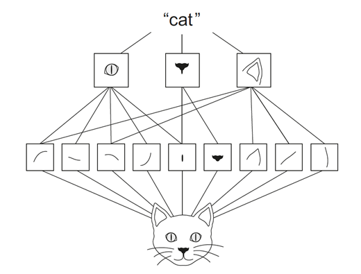
Reference Feature Extraction

Now let’s explore and understand how it’s working.

The Convolution Operation

Convolutions are operations that are applied to 3D tensors, called feature maps. These feature maps consist of two spatial axes (height and width) and a depth axis (or channels axis). If we consider the example of the RGB image, the height and width form the spatial axes and the 3 colour channels represent the depth axis. Similarly, for a black-and-white image, the depth is 1. But in the outputs of further layers, the depth is not represented by colour channels rather they stand for filters. Filters encode specific aspects of the input data i.e. a filter can encode the concept of “presence of face” or “structure of a car” etc.

The convolution operation consists of two key parameters,

1. Kernel size: The sizes of filters that are applied to the images. These are typical 3×3 or 5×5.
2. Depth of output feature map: This is the number of output filters computed by the convolution.

The convolution operation is just the multiplication and addition of weighted filters on the input feature maps to generate another 3D tensor with different widths, heights, and depth. The convolution operation works by sliding these windows of size 3×3 or 5×5  filters over 3D input feature maps, stopping at every possible location and then computing the features. We can see the operation in the following gif, the 3×3 kernel is operating on a 5×5 input feature map to generate 3×3 output.

It is important to note that the network learns the optimum filters required from the given data. The weight of the CNN model is the filters.

Now let’s look at the border effects, padding, and strides.

Understanding Border Effects and Padding

Now again let’s consider the 5×5 feature map (refer to the above gif) which has 25 tiles in total. The filter is of size 3×3 hence has 9 tiles. Now during the convolution operation, the 3×3 filter can pass through the 5×5 feature map only 9 times hence we have output with size 3×3. So the output shrinks here from 5×5 to 3×3 i.e. by two tiles alongside each dimension. Here no padding is applied to the input feature map, hence it is called valid padding.

If we want the output feature map with the same size as of input feature map, we need to use padding. Padding consists of adding an appropriate number of rows and columns on each side of the input feature map to make it possible to fit centre convolution windows around every input tile. This type of padding is called the same padding. The following GIFs represent the same padding.

Now we can see that when we add extra padding to the 5×5 feature map and apply a 3×3 filter, we will be able to get the output feature map with the same size as of input feature map.

How to find the padding to add to the given filter size and feature map?

This question naturally arises as we encounter feature maps and filters of different sizes and how can we determine how much padding we should use for valid and same cases. So to answer the question, we have the formula to determine the padding i.e.

1. Valid Padding: Since valid padding means no padding, the amount of padding will be 0.
2. Same Padding: We use the same padding to preserve the size of the input feature map. But the output of the convolution mainly depends on the filter size, regardless of the input size. Hence the padding can be determined from filter size as follows:

Same Padding = ( filter size – 1) / 2

Now let’s look at another factor that can influence the output size i.e. strides.

Understanding Strides

Stride is one of the factors that influence the size of the output feature map. Strides are the distance between two successive windows where filters are applied. In the above examples, we have seen that the filter is being applied to the input feature map as windows and is shifted by a single unit or stride. When this shift is more than one, we define it as CNN with stride. The following GIF gives an example of CNN with a stride of 2.

We can also observe when we use the value of stride as 2 (or more than one) the size of the output feature map is reduced (downsampled by a factor of 2) as compared to regular convolution ( when the value of stride = 1).

Hence we can say that using strides is one of the ways to downsample the input feature map. But they are rarely used in practice, but still, it is one of the important concepts of CNNs and it is good to know about it.

Now before going to the implementation of CNN, let’s look at another important concept used to downsample the input feature i.e. Pooling.

Understanding Pooling

Pooling operation can be defined as a way to aggressively reduce/downsample the size of the input feature map by using different strategies like taking the average, maximum, sum, etc. Let’s now look at different types of pooling

1. Max Pooling: Max-pooling is one of the widely used pooling strategies to downsample the input feature maps. In this layer, the window of definite size is passed through the input feature map and then the maximum value is obtained and is computed as the next layer or output feature map.  We can see in the below GIF, that when we perform max pooling with filter size 2, the input feature is downsampled by the factor of 2 or halved. We can determine the size of the output after using max-pooling by the below formula:

Size of output = Size of input / ( pooling filter size)

There are other kinds of pooling strategies like average pooling where the average of the window is considered and sum pooling where the sum of the weights of the window is taken into account.

But max-pooling has been the most popular and widely used pooling strategy. This is due to the fact that when we consider the maximum value from the filter window, we will be able to transfer most of the available info about the input feature/current feature map to the next feature map. Hence reducing the loss of data when we are propagating through the layers of the neural network.

Since we have some idea about how CNNs work, let’s now implement a CNN from scratch…

Training a CNN based Image Classifier from scratch

Now let’s train a CNN model on the MNIST dataset. MNIST dataset consists of images of handwritten digits from 0 to 9 i.e. as 10 classes. The training set consists of 60000 images and the test set consists of 10000 images. Let’s use CNN to train an image classifier from scratch.  We will implement the code in the Keras framework.

Keras is one of the most popular and widely used deep learning libraries. It is built as a high-level API for working with TensorFlow easily.

To follow through with the following code implementation, a Jupyter Notebook with a GPU is recommended. The same can be accessed through Google Colaboratory which provides a cloud-based jupyter notebook environment with a free Nvidia GPU.

Now let’s get started,

Getting MNIST Dataset

Before downloading the dataset, let do the necessary imports,

from tensorflow.keras.datasets import mnist

from tensorflow.keras.utils import to_categorical




from tensorflow.keras import layers

from tensorflow.keras import models




import numpy as np

import matplotlib.pyplot as plt

from matplotlib import pyplot

(train_images, train_labels), (test_images, test_labels) = mnist.load_data()

The above code downloads the data and caches it. Since we are loading a predefined dataset,  the dataset has already been preprocessed and packed in the form of a tuple. Now let’s explore the shapes of these tensors we have unpacked,

print("Shape of training dataset: ",train_images.shape)
print("Shape of test dataset: ",test_images.shape)
print("Shape of training dataset labels: ",train_labels.shape)
print("Shape of test dataset labels: ",test_labels.shape)

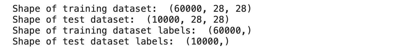
We can see from the above output, the training dataset has 60000 images, each image with a size of 28×28. similarly, the test dataset has 10000 images with an image size of 28×28. We can also see that the labels don’t have any shape i.e. it is a scalar value. Let’s look at some labels,

print(train_labels)
print(type(train_labels))

Output:

We can see that the labels are all in a single NumPy array.

Now let’s look at some of our training images,

# plot first few images
for i in range(9):
    # define subplot
    pyplot.subplot(330 + 1 + i)
    # plot raw pixel data
    pyplot.imshow(train_images[i], cmap=pyplot.get_cmap('gray'))
# show the figure
pyplot.show()

Output:

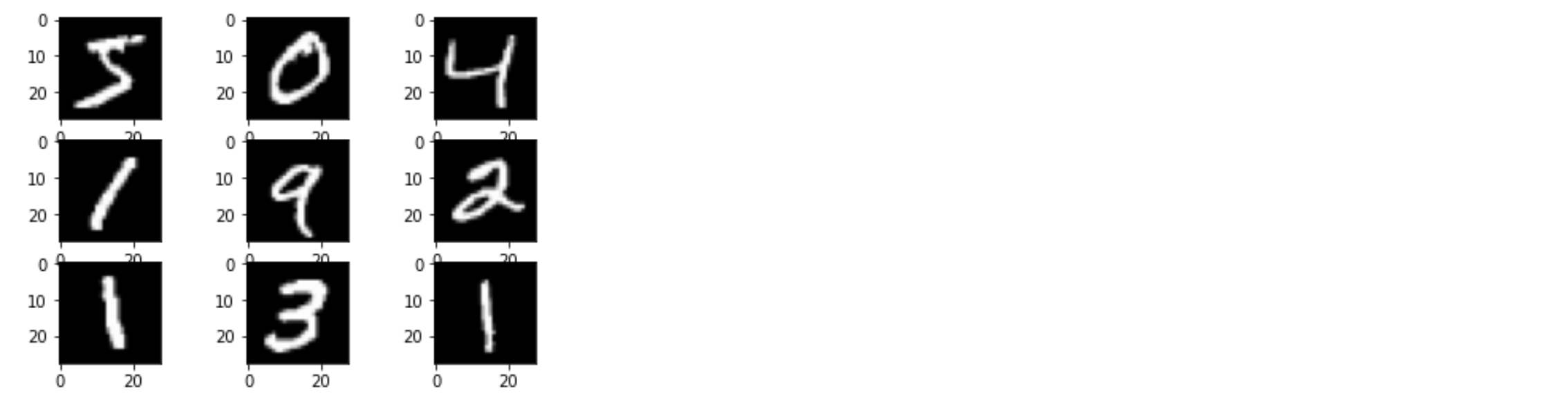
We can visualize the training samples by plotting them.

Before we proceed to model training, let do some preprocessing to our data.

Basic Preprocessing

Now let’s reshape the images to size (60000, 28, 28, 1) from (60000, 28, 28) where the last dimension represents the depth of the image. We have already seen previously that every image’s feature map will have three dimensions i.e. width, height and depth. Since the MNIST training set consists of black and white images, we can define the depth as 1.

Next, we should normalize the dataset i.e. bring all the values of the input between 0 and 1. Since the maximum value of the image layer is 255, let’s divide the entire dataset by 255.

train_images = train_images.reshape((60000, 28, 28, 1))
train_images = train_images.astype('float32') / 255

Now let’s also apply the same preprocessing to the test set.

test_images = test_images.reshape((10000, 28, 28, 1))
test_images = test_images.astype('float32') / 255

Finally, let’s convert our labels to categorical format i.e. they are currently as scalars but we are performing One-Hot encoding to uniquely map each scalar to a vector.

train_labels = to_categorical(train_labels)
test_labels = to_categorical(test_labels)

train_labels[:10]

Output:

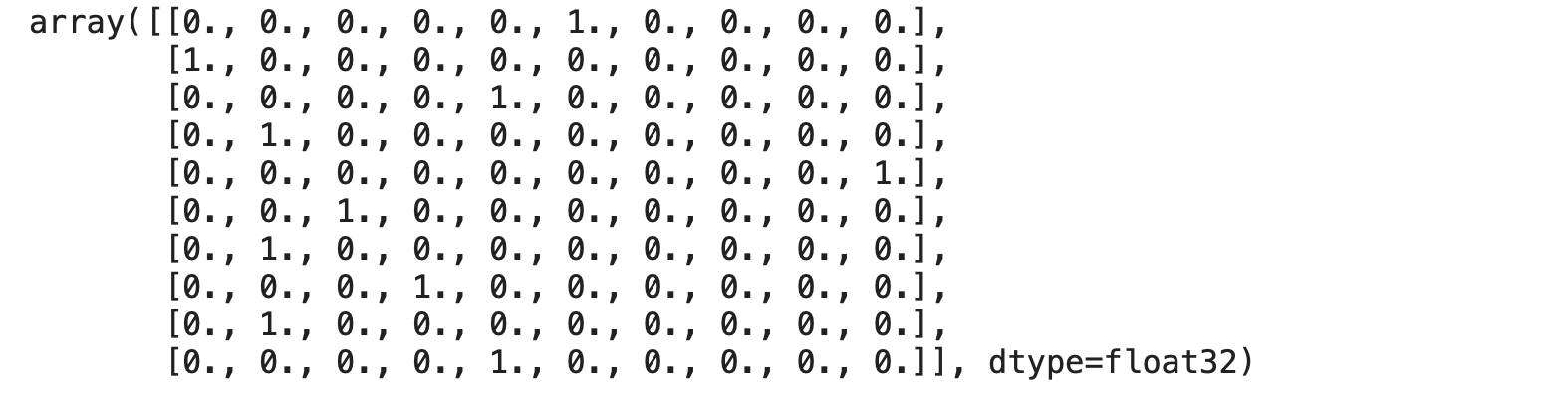
We can see that the training labels are one-hot encoded.

Now let’s create a basic CNN model using Keras.

Creating a CNN model with Tensorflow-Keras

Now let’s create a basic model using Keras library,

model = models.Sequential()
model.add(layers.Conv2D(32, (3,3), activation='relu', input_shape=(28,28,1)))
model.add(layers.MaxPool2D((2,2)))
model.add(layers.Conv2D(64, (3,3), activation='relu'))
model.add(layers.MaxPool2D((2,2)))
model.add(layers.Conv2D(64, (3,3), activation='relu'))

Now let’s analyze the above code,

• First, we are creating an object of Sequential type class. A sequential model is a type of model where we can add and stack layers to form an end-to-end model.
• Using .add we are adding the layers into our model by specifying various parameters depending on the layer.
• In the above model, we are adding a convolutional layer ( i.e. Conv2D in Keras) which accepts a number of filters, kernel size and activation function as parameters.
• Next, the max-pooling layer (i.e. MaxPool2D in Keras) is added to enable pooling operation.
• Different types of layers are available in Keras.

The above part of the model is responsible for identifying and detecting patterns present in the input data. ( The working of which we have discussed above)

Now finally let’s initialise the head by defining the number of outputs of the model.

model.add(layers.Flatten())
model.add(layers.Dense(64, activation='relu'))
model.add(layers.Dense(10, activation='softmax'))

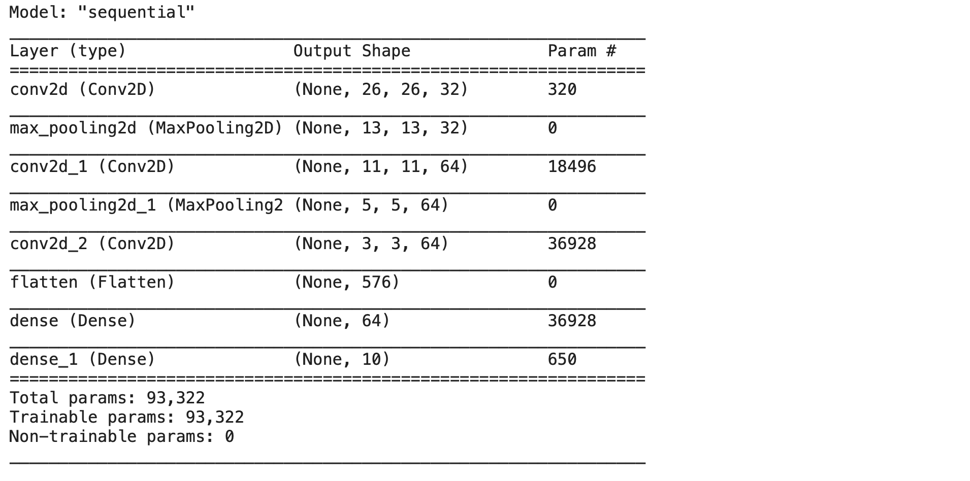
Now our model is ready. We can see the list of all layers in the model by using the .summary() method.

model.summary()

Output:

Now let’s compile the model by assigning the optimizer, loss function and metrics to use while model training.

model.compile(optimizer='rmsprop', 
              loss='categorical_crossentropy', 
              metrics=['accuracy'])

Now let’s fit the model with training data and labels and train it for 5 epochs,

model.fit(train_images, train_labels, epochs=5, batch_size=64)

Results:

 

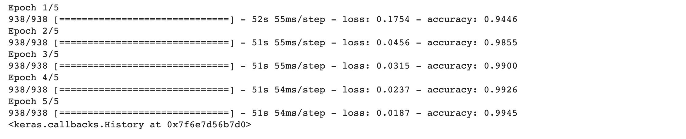
From the training results, we can see that the model was able to achieve up to 99% accuracy which is really impressive !!

Conclusion

We have seen the underlying functionality of convolutional neural networks and how it extracts features from images. Therefore we can conclude that convents are one of the techniques that produce state-of-the-art results in computer vision applications.

Thank you

References

1. Vision Image: https://www.telusinternational.com/articles/computer-vision-through-the-ages
2. Feature Extraction: https://freecontent.manning.com/deep-learning-for-image-like-data/
3. Convolution: https://medium.datadriveninvestor.com/convolutional-neural-networks-3b241a5da51e
4. Border Effects and padding: Source: https://commons.wikimedia.org/wiki/File:Convolution_arithmetic_-_Same_padding_no_strides.gif
5. Understanding strides: https://towardsdatascience.com/pytorch-basics-how-to-train-your-neural-net-intro-to-cnn-26a14c2ea29
6. Pooling:  Source: https://ai.plainenglish.io/convolutional-neural-networks-simplified-165148207e02

About Me

I’m Narasimha Karthik, a Deep Learning enthusiast.

Experience in working with PyTorch, Fastai, Tensorflow, and Keras frameworks. You can connect with me through LinkedIn or Twitter.

Thank you

Narasimha

Hi,
I am Narasimha Karthik J, a Data Scientist at Boeing Research in Bengaluru. I have experience in fine-tuning language model models (LLMs) for various domain-specific applications and deploying them. Additionally, I am experienced in LLM training, fine-tuning, RAG, and working with the latest frameworks and technologies.

Thanks and Regards,
Narasimha Karthik J