This article was published as a part of the Data Science Blogathon.
Introduction to SQL
When I was a teenager, I listed the items on paper to buy from the shop, called data in this case. In today’s world, we get lots of data through the media. So, where can we store the vast amounts of data? It’s impossible to write down all those data in a book. Suppose we use books to store those data. It is time-consuming and not easy to retrieve those data or even alter data. The information may be lost due to bad weather conditions or any misfortune. So we need a system to store the data and retrieve or update it easily.
SQL Server and Database
As I explained in the introduction, the data may be class, price, items, etc. So, data is a collection of facts, i.e., words, numbers, pictures, and a database is a repository of data. It provides functionality for adding, modifying, and querying data. A DBMS (Database Management System) is software to manage databases. One type of DBMS is RDBMS, also called a relational database management system. It is a set of software tools that control data access, organization and storage. Especially banks and healthcare use this RDBMS. Examples of RDBMS are MySQL, Oracle Database, IBM DB2, DB2 Express, and Cache.
All data models resemble its databases. The most data model used is the Relational Model. It allows for data independence. Here, data is stored in tables. It provides logical data independence, physical data independence, and physical storage independence. An entity-relationship data model is an alternative to a relational data model.
Entity-relationship data model: Here, entities are objects that exist independently of any other entities. Entities have attributes, which are the data elements that describe the entity.
For example, Book is an entity. Edition, year, price, title, etc. are attributes. An entity becomes a table, and its attributes are the columns.
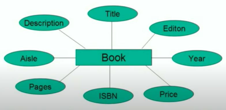
Figure 1. Entity-relationship data model
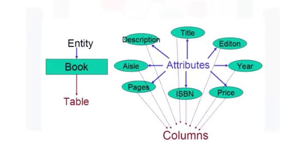
Mapping Entities to Tables: The basic foundation for designing a database Begin with an ERD (Entity-Relationship Diagram) and map the ERD to the table. Here, an entity becomes a table, and attributes are its columns that separate the entity from the attributes.
For example,
The building blocks of relational models are sets and relations.
A Relation is made up of 2 parts:
1) Relational Schema
2) Relational Instance
A Relational Schema specifies the following: the name of the relation schema, the name and type of each attribute.
Relation Instance: It is a table made up of rows and columns. Here, columns are attributes, and rows are tuples.
Degree = The number of attributes
Cardinality = The number of tuples
Relational Model Constraints
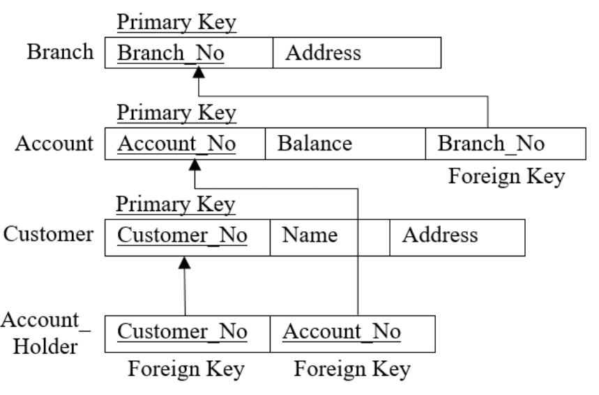
There is a mechanism to establish the data integrity between two relations In relational databases, called referencing. A primary key in a relational table uniquely identifies each row in the table. A foreign key is a set of columns referring to a primary key of another table. A table containing a primary key is related to at least one foreign key. A dependent table consists of one or more foreign keys.
In business, data must often adhere to certain restrictions, called constraints. Constraints help implement the business rules.
The following are six constraints:
1. Entity Integrity Constraints: The primary key is a unique value that identifies each row or tuple. The attribute participating in the primary key should not accept null values.
For example, BOOK_ID is a primary key that must be unique and must not be a null value in the below table.
| BOOK_ID | BOOK_NAME | BOOK_PRICE |
| B101 | Harry Potter | 1200.00 |
| B102 | My Journey | 360.00 |
| B103 | A Little Flower | 950.00 |
2. Constraints on Referential Integrity: It defines relationships between tables and ensures that they remain valid. The validity of the data is enforced using a combination of primary key and foreign key.
For example,
3. Semantic Integrity Constraints: It is related to the correctness of the data.
For example, All columns should not contain garbage values like @, *, % and so on in the below table.
| BOOK_ID | BOOK_NAME | BOOK_PRICE |
| B101 | Harry Potter | 1200.00 |
| B102 | My Journey | 360.00 |
| B103 | A Little Flower | 950.00 |
4. Domain Constraints: It allows valid values for a given attribute.
For example, BOOK_NAME must be characters, and BOOK_PRICE must be numeric in the below table.
| BOOK_ID | BOOK_NAME | BOOK_PRICE |
| B101 | Harry Potter | 1200.00 |
| B102 | My Journey | 360.00 |
| B103 | A Little Flower | 950.00 |
5. Null Constraints: Attribute values are not allowed to be null.
For example, BOOK_NAME must not be null in the below table.
| BOOK_ID | BOOK_NAME | BOOK_PRICE |
| B101 | Harry Potter | 1200.00 |
| B102 | My Journey | 360.00 |
| B103 | A Little Flower | 950.00 |
6. Check Constraints: It is a rule or a set of rules which helps check the inserted (or updated) data values in tables based on a condition.
For example, BOOK_PRICE must not be negative values in the below table.
| BOOK_ID | BOOK_NAME | BOOK_PRICE |
| B101 | Harry Potter | 1200.00 |
| B102 | My Journey | 360.00 |
| B103 | A Little Flower | 950.00 |
Types of SQL Statements
SQL statements, namely, DDL and DML.
1. DDL (Data Definition Language): These statements are used to create, modify, or delete database objects, such as tables. Examples, are create, alter, truncate, and drop.
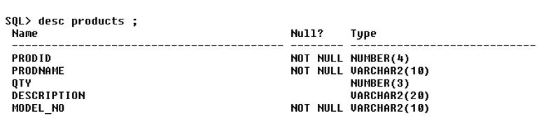
i. Create: This statement is used to create tables and define their columns. Note that the basic data types we use in SQL are char, varchar, number, date, clob.
Syntax:
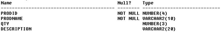
create table
(column_name_1 datatype optional_parameters, column_ name_2 datatype, ……………., column name_n datatype) Code: create table products(PRODID number(4) primary key, PRODNAME varchar(10) not null, QTY number(3) check (qty > 0), DESCRIPTION varchar(20));Output:
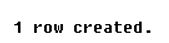
ii. Alter: This statement is used for altering tables, including adding and dropping columns and modifying their data types.Syntax: alter tableadd column_name datatype;Code:
alter table products add MODEL_NO varchar(10) not null;Output:
iii. Truncate: This statement is used for deleting data in a table but not the table itself.
Syntax: truncate table; Code: truncate table test; iv. Drop: This statement is used for deleting the table itself.Syntax: drop table;Code: drop table test;
2. DML (Data Manipulation Language): These statements are used to modify data in a table. Examples for DML are: create, read, update, and delete.i. Insert statement: It populates the table with data. It is a data manipulation language statement used to read and modify data.Syntax: Insert into () values ();
Code:
insert into products (PRODID, PRODNAME, QTY_ AVAILABLE, DESCRIPTION) values (1002, ‘Laptop’, 23, ‘Dell’);
Output:
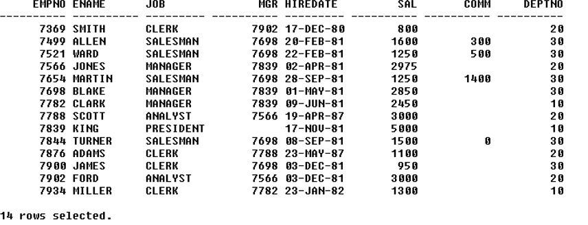
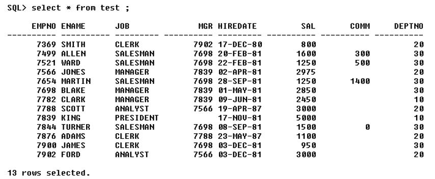
ii. Select statement and where clause: It is a data manipulation language used to read and modify data.
Syntax: select * fromCode: select * from emp;Output:
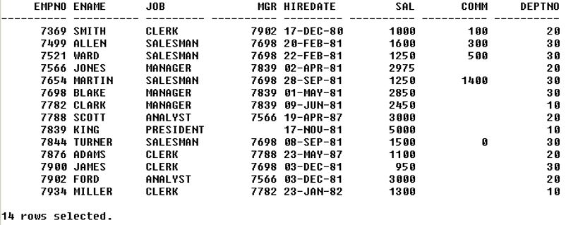
iii. Update statement: It is a data manipulation language statement used to read and modify data.Syntax: update set [[columnname]=[value]] whereCode: update emp set sal=sal+200, comm=100 where empno = 7369;Output:
iv. Delete statement: It is a data manipulation language used to read and modify data. Syntax: delete from whereCode: select * from test;Output:

Code: delete from test where empno=7934;Output:
Group functions and Grouping1. Group functions: There are 5 group functions. They are sum, max, min, avg and count.
- sum: It returns the total value
- max: It returns the maximum value
- min: It returns a minimum value
- avg: It returns the average value
- count: It returns the number of records
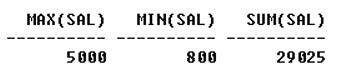
code:
select max(SAL), min(SAL), sum(SAL) from emp; Output:
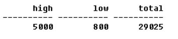
we can give names to the group functions.code: select max(SAL) as “high”, min(SAL) as “low”, sum(SAL) as “total” from emp;Output:
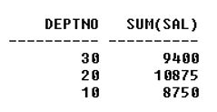
2. Grouping: It is a process of computing the aggregates by aggregating based on one or more columns. Grouping is generated by using the ‘group by’ clause. Syntax: select , , …….., [Group functions] from group by , …….,Code: select DEPTNO, sum(SAL) from emp group by DEPTNO;Output:
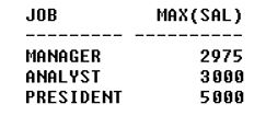
3. having, where clause and order by: ‘having’ is used to filter the grouped data and ‘where’ is used to filter the non-grouped data. ‘where’ should be used before group by clause and having should be used after group by clause. ‘order by’ is used at the end of the statement.
Syntax: select [column names] from where group by having order by ;Code: select job, max(sal) from emp where deptno 30 group by job having max(sal)>1500 order by 2;Output:
Conclusion
In this article, we have learned
- How to map entities and attributes into tables.
- We saw the relational model and its constraints are rules for adding data to a table.
- Also, We have learned to make necessary changes in the schema using the DDL statements and DML statements for creating and updating the table.
- Finally, we saw Grouping, and filtering statements for data analysis.
I hope you found this article useful. Several programming languages like Python, R, Scala, and SAS use SQL syntax. Data Analytics uses SQL for analysis. Even we can use SQL in machine learning algorithms. I hope, you will see this in my next article.
The media shown in this article is not owned by Analytics Vidhya and is used at the Author’s discretion.


