This article was published as a part of the Data Science Blogathon.
An autoencoder is a neural network model that learns to encode data and regenerate the data back from the encodings. The input data usually has a lot of dimensions and there is a necessity to perform dimensionality reduction and retain only the necessary information. An autoencoder contains two parts – encoder and decoder. As the name suggests, the encoder performs encoding (dimensionality reduction) and the decoder tries to regenerate the original input data from the encodings. Dimensionality reduction, image compression, image denoising, image regeneration, and feature extraction are some of the tasks autoencoders can handle. An extension of autoencoder known as variational autoencoder can be used to generate potentially a new image dataset from an available set of images.
We will learn the architecture and working of an autoencoder by building and training a simple autoencoder using the classical MNIST dataset in this article. Let’s get started.
The classical MNIST dataset contains images of handwritten digits. It consists of 60,000 training and 10,000 testing images in the dataset. Each image in the dataset is square and has (28×28) 784 pixels in total. The MNIST dataset is so popular that it comes bundled directly with many python packages like TensorFlow and sklearn. We will be directly importing the dataset from TensorFlow in this project.
We will be using TensorFlow and Keras for building and training the autoencoder.
import tensorflow as tf
from keras import backend as K
import keras
import numpy as np
from tensorflow.keras import layers
from tensorflow.keras.models import Sequential
import matplotlib.pyplot as plt
The MNIST dataset can be directly accessed and loaded from TensorFlow. Essentially, the class labels for the images are not used for training the autoencoder and could be safely dropped but I will be using them to label the plots for better understanding. We will normalize the images to reduce the computational complexity of training the autoencoder. The 1 present in the output after reshaping refers to the number of channels present in the image. As we are dealing with grayscale images, the number of channels will be 1.
# loading mnist dataset
(x_train, y_train), (x_test, y_test) = keras.<a onclick="parent.postMessage({'referent':'.keras.datasets'}, '*')">datasets.mnist.load_data()
# normalising and reshaping the data
x_train = x_train.astype('float32') / 255.
x_test = x_test.astype('float32') / 255.
x_train = np.<a onclick="parent.postMessage({'referent':'.numpy.reshape'}, '*')">reshape(x_train, (x_train.shape[0], 28, 28, 1))
x_test = np.<a onclick="parent.postMessage({'referent':'.numpy.reshape'}, '*')">reshape(x_test, (x_test.shape[0], 28, 28, 1))
x_train.shape, x_test.shape
((60000, 28, 28, 1), (10000, 28, 28, 1))
As mentioned earlier, the autoencoder is made up of two parts – encoder and decoder. The architecture of the encoder and decoder are mirror images of one another. For example, the encoder has max-pooling layers to reduce the dimension of the features while the decoder has upsampling layers that increase the number of features. We will build and train the autoencoder and later extract the encoder and decoder from the layers of the trained autoencoder. We will be using the functional API for building the autoencoder. The functional API provides better control to the user for building the autoencoder. The encoder part of the autoencoder will have three Convolution – Rectified Linear Unit – MaxPooling layers. The input for the encoder will be the 28×28 grayscale image and the output will be the 4x4x8 (or 128) feature encoding. The encoder will reduce the number of features from 784 to 128. So, essentially each image consisting of 784 features will be represented efficiently using just 128 features. The encoder can be used separately as a dimensionality reducer replacing methods like PCA, BFE, and FFS to extract only the important features. As mentioned earlier, the decoder’s architecture will be the mirror image of the encoder’s architecture. So, the decoder part will have three Convolution – Rectified Linear Unit – Upsampling layers. As the pooling layers perform dimensionality reduction in the encoder, upsampling layers will increase the number of features and hence are used in the decoder. The upsampling layer does not interpolate new data but simply repeats the rows and columns thereby increasing the dimension for the regeneration process. You can learn more about upsampling layer used in this article here. The decoder will try to reproduce the input image from the 128-feature encoding. The input for the decoder will be the 4x4x8 (or 128) feature encodings produced by the encoder and the output of the decoder will be the 28×28 grayscale image. The difference between the regenerated image by the decoder and the original input image will be the loss which will be backpropagated to train the autoencoder.
input_img = keras.<a onclick="parent.postMessage({'referent':'.keras.Input'}, '*')">Input(shape=(28, 28, 1))

x = layers.<a onclick="parent.postMessage({'referent':'.tensorflow.keras.layers.Conv2D'}, '*')">Conv2D(32, (3, 3), activation='relu', padding='same')(input_img)
x = layers.<a onclick="parent.postMessage({'referent':'.tensorflow.keras.layers.MaxPooling2D'}, '*')">MaxPooling2D((2, 2), padding='same')(x)
x = layers.<a onclick="parent.postMessage({'referent':'.tensorflow.keras.layers.Conv2D'}, '*')">Conv2D(16, (3, 3), activation='relu', padding='same')(x)
x = layers.<a onclick="parent.postMessage({'referent':'.tensorflow.keras.layers.MaxPooling2D'}, '*')">MaxPooling2D((2, 2), padding='same')(x)
x = layers.<a onclick="parent.postMessage({'referent':'.tensorflow.keras.layers.Conv2D'}, '*')">Conv2D(8, (3, 3), activation='relu', padding='same')(x)
encoded = layers.<a onclick="parent.postMessage({'referent':'.tensorflow.keras.layers.MaxPooling2D'}, '*')">MaxPooling2D((2, 2), padding='same')(x)

# the shape is 4,4,8 here

x = layers.<a onclick="parent.postMessage({'referent':'.tensorflow.keras.layers.Conv2D'}, '*')">Conv2D(8, (3, 3), activation='relu', padding='same')(encoded)
x = layers.<a onclick="parent.postMessage({'referent':'.tensorflow.keras.layers.UpSampling2D'}, '*')">UpSampling2D((2, 2))(x)
x = layers.<a onclick="parent.postMessage({'referent':'.tensorflow.keras.layers.Conv2D'}, '*')">Conv2D(16, (3, 3), activation='relu', padding='same')(x)
x = layers.<a onclick="parent.postMessage({'referent':'.tensorflow.keras.layers.UpSampling2D'}, '*')">UpSampling2D((2, 2))(x)
x = layers.<a onclick="parent.postMessage({'referent':'.tensorflow.keras.layers.Conv2D'}, '*')">Conv2D(32, (3, 3), activation='relu')(x)
x = layers.<a onclick="parent.postMessage({'referent':'.tensorflow.keras.layers.UpSampling2D'}, '*')">UpSampling2D((2, 2))(x)
decoded = layers.<a onclick="parent.postMessage({'referent':'.tensorflow.keras.layers.Conv2D'}, '*')">Conv2D(1, (3, 3), activation='sigmoid', padding='same')(x)

autoencoder = keras.<a onclick="parent.postMessage({'referent':'.keras.Model'}, '*')">Model(input_img, decoded)
autoencoder.compile(optimizer='adam', loss='binary_crossentropy')
autoencoder.summary()
This is the overall architecture of the autoencoder.
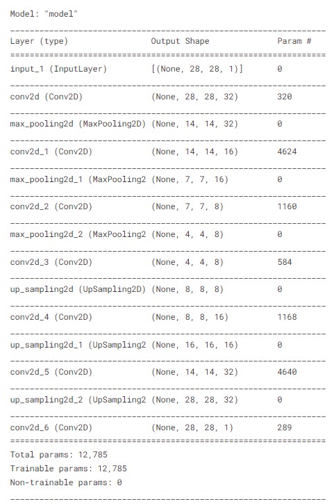
Architecture of the autoencoder
As mentioned earlier, both the input and the output will be the same for autoencoders. So, the images will be the input and output for training the autoencoder.
autoencoder.fit(x_train, x_train, epochs=100, batch_size=128, validation_data=(x_test, x_test))
Epoch 1/100
469/469 [==============================] - 33s 67ms/step - loss: 0.1892 - val_loss: 0.1296
Epoch 2/100
469/469 [==============================] - 30s 65ms/step - loss: 0.1214 - val_loss: 0.1136
Epoch 3/100
469/469 [==============================] - 30s 63ms/step - loss: 0.1112 - val_loss: 0.1070
...
...
Epoch 99/100
469/469 [==============================] - 30s 64ms/step - loss: 0.0808 - val_loss: 0.0798
Epoch 100/100
469/469 [==============================] - 31s 65ms/step - loss: 0.0808 - val_loss: 0.0798
The first 7 layers represent the encoder while the remaining layers represent the decoder. We can extract the respective layers from the trained autoencoder and build the encoder and decoder.
encoder = Sequential()
decoder = Sequential()
for layer in autoencoder.layers[:8]: encoder.add(layer)
for layer in autoencoder.layers[8:]: decoder.add(layer)
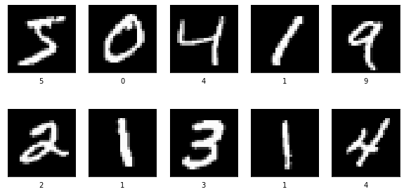
These are the first ten samples from the training set.
plt.figure(figsize=(10,5))
n = 10
for i in range(n):
plt.subplot(2,5,i+1)
plt.xticks([])
plt.yticks([])
plt.grid(False)
plt.imshow(x_train[i], cmap='gray')
plt.xlabel(y_train[i])
plt.show()
samples input images
To understand how the encoder and decoder work, we will use them separately to encode and then decode the samples. We will first encode the sample input images into 128-feature encodings using the encoder. Then, we will use the decoder to regenerate the input images from the 128-feature encodings created by the encoder.
encoded_sample = encoder.predict(x_train[0:10]) # encoding
encoded_sample.shape
(10, 4, 4, 8)
decoded_sample = decoder.predict(encoded_sample) # decoding
decoded_sample.shape
(10, 28, 28, 1)
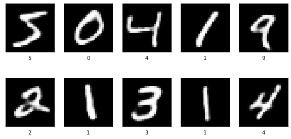
These are the generated images by the decoder using the 128-feature encodings from the encoder.
plt.figure(figsize=(10,5))
n = 10
for i in range(n):
plt.subplot(2,5,i+1)
plt.xticks([])
plt.yticks([])
plt.grid(False)
plt.imshow(decoded_sample[i], cmap='gray')
plt.xlabel(y_train[i])
plt.show()
decoder generated images
We can see that the autoencoder is able to regenerate images accurately. Now, let us try to generate a new set of images. Essentially, variational autoencoders need to be used for this purpose. Autoencoders can be used for generating new images but the drawback is that they might produce a lot of noise if the encodings are too different and non-overlapping.
For generating a new set of images, we need to interpolate new encodings and use them to generate new images using the decoder. We will use the first two pictures shown in the sample input images and see how the digit 5 can be changed to digit 0.
starting, ending = encoder.predict(x_train[0:2])
# interpolating new encodings
values = np.linspace(starting, ending, 10)
generated_images = decoder.predict(values) # generate new images
plt.figure(figsize=(10,5))
n = 10
for i in range(n):
    plt.subplot(2,5,i+1)
    plt.xticks([])
    plt.yticks([])
    plt.grid(False)
    plt.imshow(generated_images[i], cmap='gray')
plt.show()
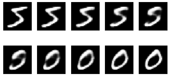
We can see how a new set of images are being generated by the encodings that we interpolated.
In this article, we discussed the following.
For generating new images by interpolating new encodings, we can use variational autoencoders. Variational autoencoders use the KL-divergence loss function which ensures that the encodings overlap and hence the process of generating new images is much smoother, noise-free, and of better quality. This is the reason why variational autoencoders perform better than vanilla autoencoders for generating new images. I will try to cover variational autoencoders in another article. That’s it for this article.
Thanks for reading and happy learning!
The media shown in this article is not owned by Analytics Vidhya and is used at the Author’s discretion.
Lorem ipsum dolor sit amet, consectetur adipiscing elit,


