Backward Feature Elimination and its Implementation

Introduction

In the previous article, we saw another feature selection technique, the Low Variance Filter. So far we’ve seen Missing Value Ratio and Low Variance Filter techniques, In this article, I’m going to cover one more technique use for feature selection know as Backward Feature Elimination.

Let’s Begin!

Note: If you are more interested in learning concepts in an Audio-Visual format, We have this entire article explained in the video below. If not, you may continue reading.

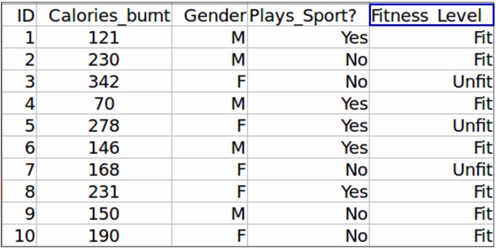
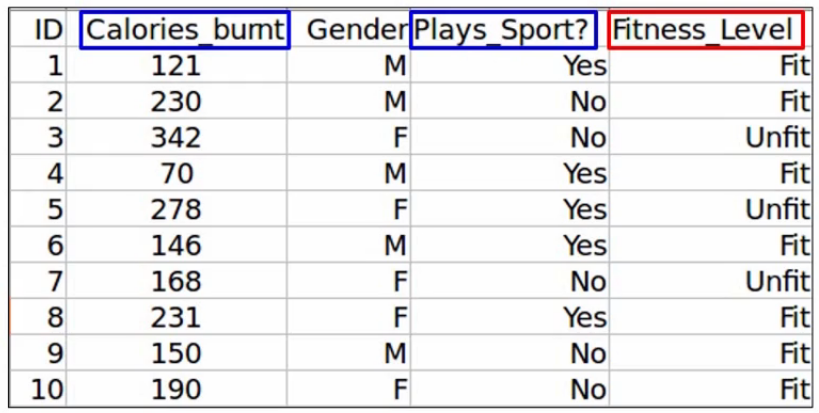
Let’s say we have the same problem statement where we want to predict the fitness level based on the given feature-

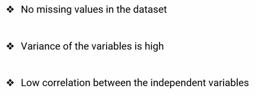
Let’s assume we don’t have any missing values in the dataset. Also, the variance of all the variables is high and the relation between the independent variables is low. These are our assumptions-

So there’s one more technique called Backward Feature Elimination that we can use to select the important features from the dataset. Let’s look at the steps to perform backward feature elimination, which will help us to understand the technique.

The first step is to train the model, using all the variables. You’ll of course not take the ID variable train the model as ID contains a unique value for each observation. So we’ll first train the model using the other three independent variables. And of course, the target variable, which is the Fitness_Level.

Next, we will calculate the performance of the model. Let’s say we get an accuracy of 92% using all three independent variables.

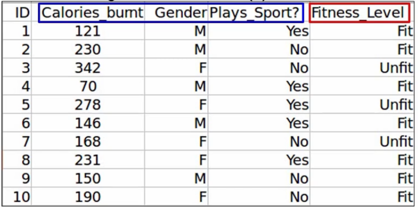
Next, we will eliminate a variable and train the model on the remaining variables. So let’s say we drop the Calories_Burnt variable and trained the model on the remaining two variables, Gender, and Plays_Sport. Now we will calculate the performance in the model on this new data, which is after dropping that one variable, we get an accuracy of 90% after dropping the Calories_Burnt variable-

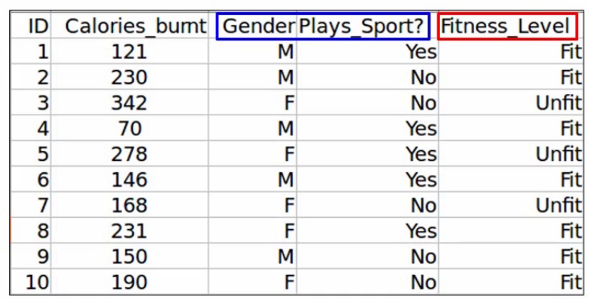
Similarly, we will drop each variable at a time and train the model on the remaining variables. Here we’ve dropped the Gender variable, as you can see-

and we get an accuracy of 91.6%. Finally, we drop the Plays_Sport variable, and again, train the model on the remaining data-

and get an accuracy of 88% a slight drop. Now, once the model is trained after dropping each variable at a time, we will identify the eliminated variable, which perhaps did not impact the performance as much.

So if you recall, we got an accuracy of 92% when we used all the variables, and here is the accuracy after dropping each variable-

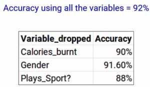
So when we dropped Calories-Burnt, we got an accuracy of 90%. When we drop the Gender, we got 91.6%. And when we drop Plays_Sport, the accuracy dropped even further to 88%. If you see gender has produced the smallest change in the performance in the model first, it was 92% when we took all the variables and when we dropped gender, it was 91.6%. So we can infer that gender does not have a high impact on the Fitness_Level variable. And hence it can be dropped.

Finally, we will repeat all these steps until no more variables can be dropped. I hope you got a very good sense of how backward feature elimination works. It’s a very simple, but very effective technique.

Implementation

Now we will see how to implement it in Python. First import Pandas. I’m sure you must have learned this off by heart at this point-

#importing the libraries
import pandas as pd

Next, read the dataset and print the first five observations using the data.head() function-

#reading the file

data = pd.read_csv('backward_feature_elimination.csv')
data.head()

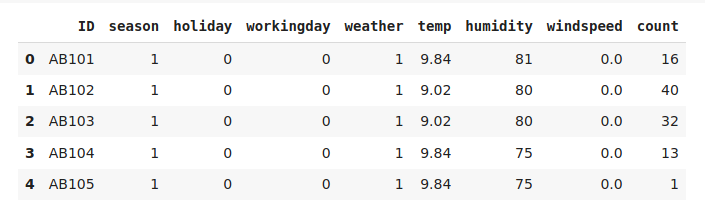
We have the target variable and the other independent variables. Let’s see the shape of our data-

#shape of the data
data.shape

12,980 observations and 9 columns of variables. Let’s check. If there are any missing values are not-

# checking missing values in the data
data.isnull().sum()

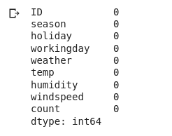
There aren’t, Perfect! Now since we will be training a model on our data set, we need to explicitly define the target variable and the independent variables-

# creating the training data

X = data.drop(['ID', 'count'], axis=1)
y = data['count']

X here will be the independent variables after dropping the ID variable and y will be the target variable, “count”. Let me print the shape of both of these-

X.shape, y.shape

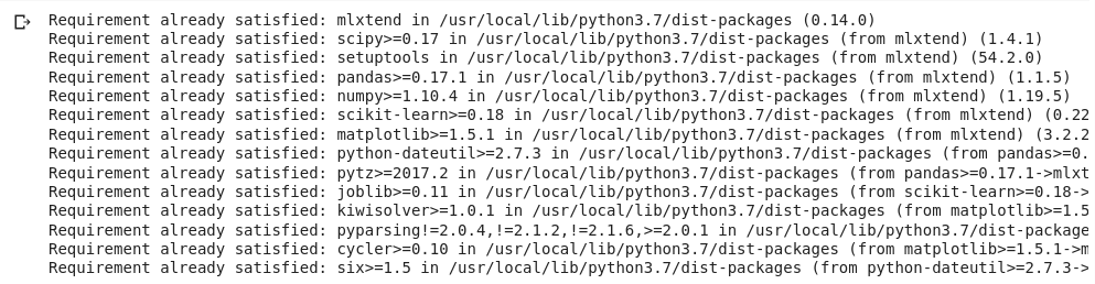
and it looks perfect. Now, this is very important. We need to install “the mlxtend” library, which has pre-written codes for both backward feature elimination and forward feature selection techniques. This might take a few moments depending on how fast your internet connection is-

!pip install mlxtend

All right, we have it installed here. Now from the recently installed mlxtend, we’ll import the SequencialFeatureSelector from the sklearn library we’ll important LinearRegression. Why? Because you’re working on a regression problem, where we have to predict the count of bikes rented-

from mlxtend.feature_selection import SequentialFeatureSelector as sfs
from sklearn.linear_model import LinearRegression

Let’s go ahead and train our model. Here, we’ll first call the linear regression model and then we define the feature selector model-

lreg = LinearRegression()

sfs1 = sfs(lreg, k_features=4, forward=False, verbose=1, scoring='neg_mean_squared_error')

Let me explain the different parameters that you’re seeing here. The first parameter here is a model name and hence I’ve passed lreg here, which is the linear regression model.

Then we have to define how many features should be selected. For our example I’ve passed “k_features = 4”, so the model will train until only four features are left.

Next “forward = False” here means that we are training the backward feature elimination and not the forward feature selection method.

The next “verbose = 1” will allow us to print the model summary at each iteration.

And finally, as this is a regression model, scoring will be based on the mean squared error metric hence “scoring = ‘neg_mean_squared_error'”.

Let’s go ahead and fit the model here-

sfs1 = sfs1.fit(X, y)

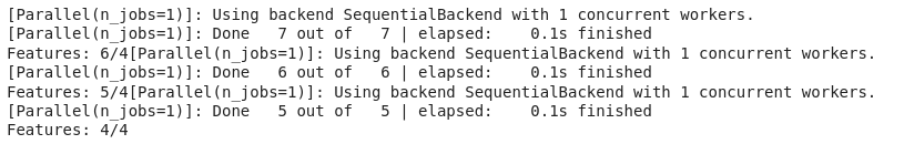
We can see that the model was trained until finally only four features are left. Let’s go ahead and print the features that have been selected-

feat_names = list(sfs1.k_feature_names_)
print(feat_names)

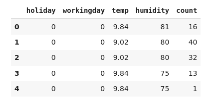
These are the selected variables. We’ll put these variables into a new data frame and print the first five observations. So let me go ahead and do that-

new_data = data[feat_names]
new_data['count'] = data['count']

new_data.head()

Here we go! Let’s just compare the shape of two datasets-

# shape of new and original data
new_data.shape, data.shape

Comparing the shape of the two datasets confirms that we have successfully implemented this method.

End Notes

This was all about Backward Feature Elimination.

If you are looking to kick start your Data Science Journey and want every topic under one roof, your search stops here. Check out Analytics Vidhya’s Certified AI & ML BlackBelt Plus Program

If you have any queries let me know in the comment section!

Himanshi Singh

I’m a data lover who enjoys finding hidden patterns and turning them into useful insights. As the Manager - Content and Growth at Analytics Vidhya, I help data enthusiasts learn, share, and grow together. 

Thanks for stopping by my profile - hope you found something you liked :)