Customer Churn Prediction of a Telecom Company Using Python

This article was published as a part of the Data Science Blogathon.

Introduction to Customer Churn Prediction

After taking some courses on Data Science, I feel a necessity for applying those skills to some projects. For this, I analyzed and made a machine learning model on a dataset that comes from an Iranian telecom company, with each row representing a customer over a year period. I took this dataset from Kaggle. In this article, I am going to share my experience while working with this data. You will learn about

• Retrieving data from a database
• Handling imbalanced data
• Data Visualization
• Making a machine learning model

Importing Necessary Libraries for customer churn Prediction

Before starting the analysis, we have to import some libraries. The required libraries are listed below.

Retrieving Data from a Database

After taking the data from Kaggle, I push those data into a database for practicing a little bit of SQL while doing this project. You can find the database and the data as a CSV from my Github repo. Here I am using an SQLite database for simplicity. For reading an SQLite database, there is already a library called sqlite3 in python. First, let’s see how many tables are there in our database.

if we run the above code, you can see the output something like that.

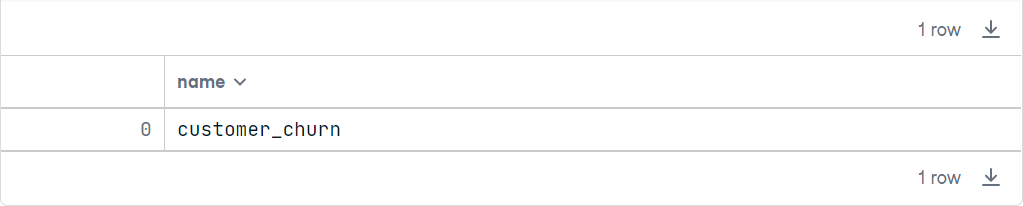
We can see from the above result that there is only one table in that database. That makes sense as I only pushed one table into the database. Now let’s see the structure of the customer_churn table. For this, we have to run the code below.

If we run this code, the output will look like the below image.

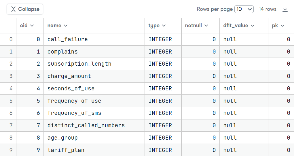
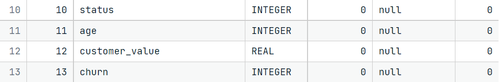
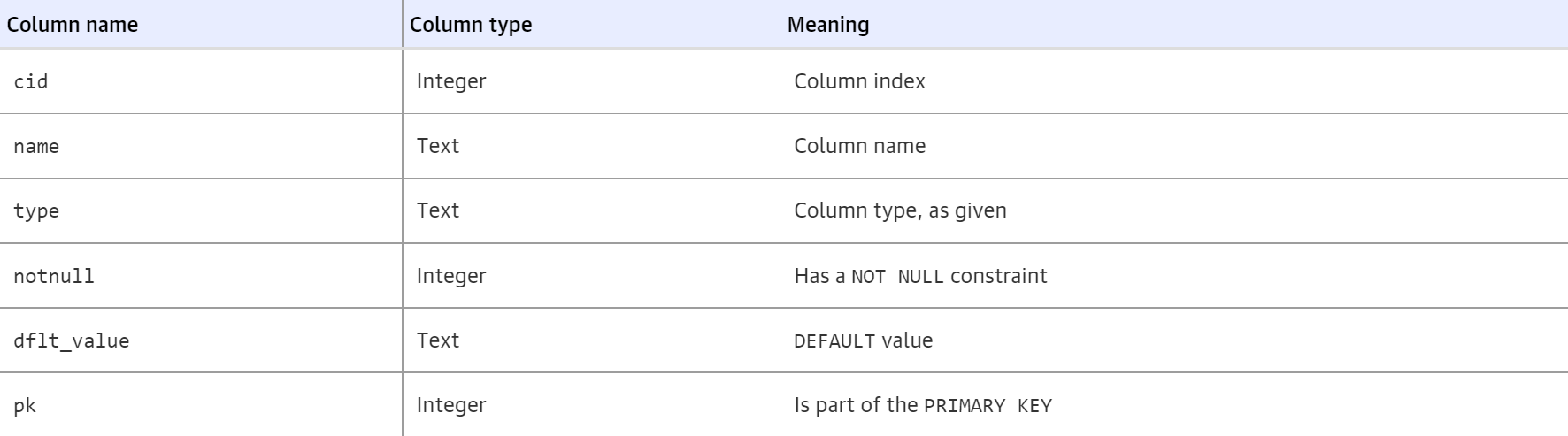
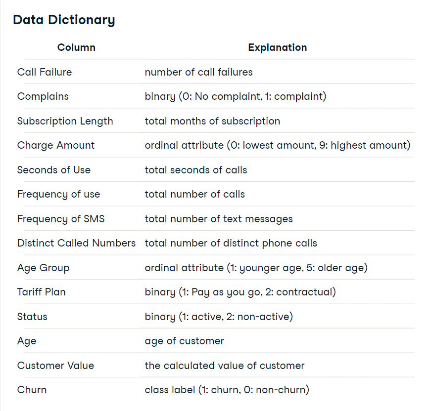
The meaning of all columns of the above table is given below:

So, from our result, we can say that:

• There are 14 columns in our table (row count of the table).
• All columns consist of either INTEGER or REAL data types (type column).
• There is no column in which the NOT NULL constraint is applied while making this table (notnull column).
• The default value is all column is null (dflt_value column).
• There is no primary key available (pk column).

We came to know so many things in just 1 line of code, isn’t that awesome?

Now, let’s see some values in the table. Run the below code.

pd.read_sql("SELECT * FROM customer_churn LIMIT 10", conn)

You will see the output something like this.

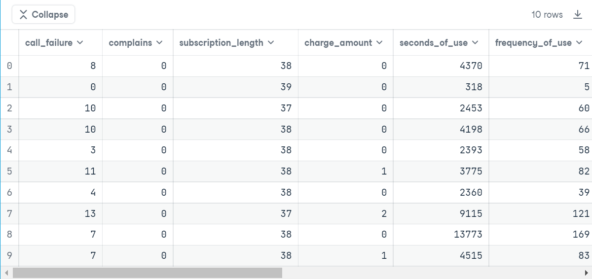
As there are so many columns, I am unable to display all of them. But I will give you a brief description of all the columns and their values to better understand the data. Just see the below image.

From the above image, you already guessed that though all columns are numerical, some encoded categorical columns exist. the encoded categorical columns are –  Complaints, Charge Amount, Age Group, Tariff Plan, Status, and Churn. The Churn column is the target column here.

Now, it’s time for reading this dataset as a pandas dataframe. But we don’t take all columns.

• There are two columns on age. So we only take Age Group here because before feeding the data into the machine learning model, we have to encode that column which is already done here.
• We are ignoring call_failure, subscription_length, charge_amount, and tariff_plan as they are not so useful for determining customer churn.

Now, let’s write the code.

Now our data is ready to do some serious analysis.

Data Analysis for Customer Churn Prediction

Now, let’s look into the summary statistics for the numerical columns.

tel_data[["seconds_of_use", "frequency_of_use", "frequency_of_sms", "customer_value"]].describe()

this code will give us the below output:

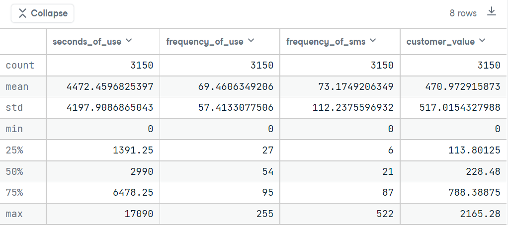
From the above statistics, we can easily notice that all numerical columns have a minimum value of 0. They may be the new customers or the missing values of these columns are present in those columns as 0. Which one is true🤨? Let’s find out.

assert 
tel_data[tel_data['seconds_of_use'] == 0].shape[0] == 
tel_data[tel_data['frequency_of_use'] == 0].shape[0]

if we run the above code, we got nothing as output. it may happen that these two columns – seconds_of_use and frequency_of_use– carry the same importance in the data. Now we have to find out that the frequency_of_sms columns are 0 too where these two columns are 0? Let’s see🔍.

If you run the above code, you will see the below two plots.

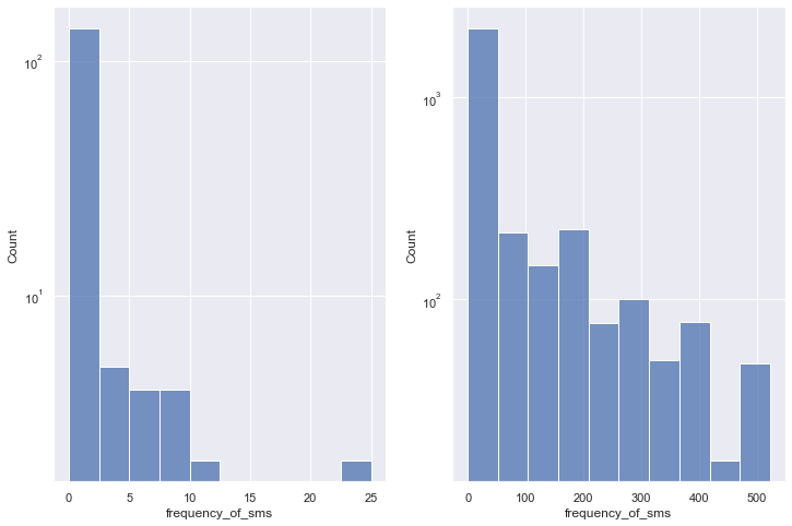
We can easily notice the difference between the above two plots. The left plot is drawn on that part of the dataset where seconds_of_use and frequency_of_use columns contain the value zero. The other one is drawn on the whole dataset. The first plot has the max value of SMS is 25 but in the other plot, this max value is more than 500! so we now came to the inference that the zero values in those columns are not missing values, those indicate that they are the new customers. Otherwise, we don’t see any bar in the left plot.

Now, you may notice that I used a log scale on the y-axis while plotting. Why? Because of the large difference between the values in the frequency_of_sms column. if there is a large value difference in a column and we plot those values without using a log scale, it is very hard to come into some inference from the plot. So we have to use a log scale when we face such a problem.

Now, this data contains 8 columns. Are all of them important? Let’s see by finding the correlation matrix.

We got the image below as an output.

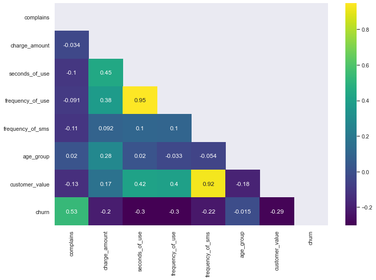
From the correlation matrix, we can easily notice that

• frequency_of_use and seconds_of_use have a high positive correlation between them. So we can put any one of them in the data.

I am removing the frequency_of_use column from the data.

tel_data_selected = tel_data.drop('frequency_of_use', axis=1)

Dealing with Imbalance

Here we want to predict the churned customers properly. Let’s see how many rows are available for each class in the data.

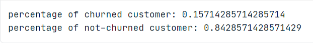
The output

Hmm, only 15% of data are related to the churned customers and 84% of data are related to the non-churned customer. That’s a great difference. We have to oversample the minority class. For doing this, I am using SMOTE(Synthetic Minority Over-sampling TechniquE) which makes synthetic data using the characteristics of the nearest neighbours. This technique is available in the imblearn python library.

There is also one thing. We don’t want to test the ml model on fake data! So I am using this technique only on the training data. For this, we are splitting the data using train_test_split from scikit-learn.

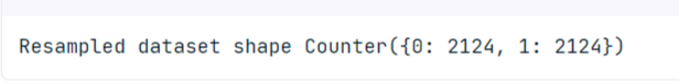
Now our data is balanced. There is one more thing to do before training a model –  Scaling the numeric data. seconds_of_use, frequency_of_sms, and the customer_value columns are the numeric columns. Other columns are encoded categorical columns. So we have to scale only these 3 columns. For selecting the specific column for scaling I am using ColumnTransformer from scikit-learn and StandardScaler for scaling. 

To know about the ColumnTransformer, see here.

Training a Model

Now it’s the time for model training. Here I am using the LogisticRegression for classification.

I don’t make the model much more complex here so that a beginner can easily understand it. I am using all the default hyperparameters for Logistic Regression.

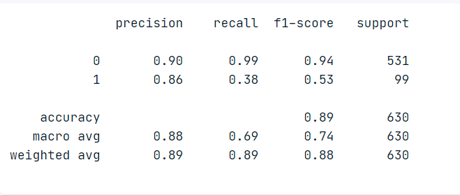
Now we have to check that this default model works well in predicting the churned customer. As we are only interested in a specific class here, so I am using recall as an evaluation metric. Recall calculates the percentage of actual positives a model correctly identified (True Positive). Here we are predicting the churned customers which are our positive class. Let’s see what we got.

from sklearn.metrics import classification_report, ConfusionMatrixDisplay
print(classification_report(y_test, y_pred))

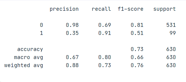
The output

From the above classification report, we can see that the model gives a decent score for predicting the customer as churned, which is great!

Now, let’s plot the Confusion Matrix.

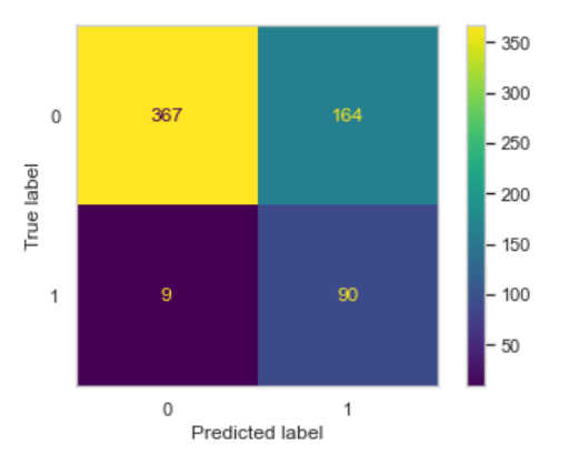
From the 99 churned customer samples, we are detecting 90 samples correctly and 9 are misclassified. This result might change in multiple reruns.

What happens if we just pass the data without resampling? Let’s see.

Now we are getting a bad recall score. What about the Confusion Matrix? Let’s see.

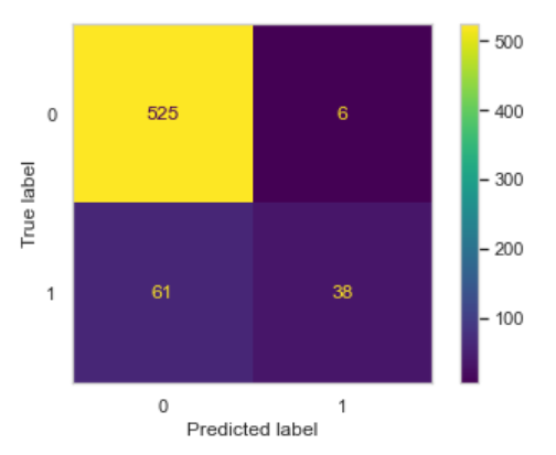
From the confusion matrix, we can see that this model is not working well for detecting the churned customer.

Conclusion

So, we can see from the above result that here the resampling technique gives a better result in predicting the churned customers. And from the analysis, we can see that not all features are important here. I take only 6 features out of 14 features but still model gives a decent result. You can also try the other features too, the journey does not end here.

This model can be improved by tuning the hyperparameters or using other algorithms other than LogisticRegression. We can also apply Cross-Validation for taking the best split of the data for training.

That’s all for now. I hope you enjoyed reading this article. Thanks for reading this article so far😁. But for now, Sayonara👋.

The media shown in this article is not owned by Analytics Vidhya and is used at the Author’s discretion.