Introduction
This article explores the potential of machine learning in understanding critical indicators of heart disease prediction. Heart disease puts an enormous burden on the global healthcare system. Many adverse events could have been prevented if the problem had been resolved on time. Machine learning holds promise in diagnosing the possibility of adverse cardiac outcomes in high-risk individuals.
This article will use the “personal key indicators of heart disease” dataset to identify individuals at risk for heart disease. The dataset comprises an annual survey by the CDC (Center for Disease Control) in the USA concerning 400000 adults’ health status. The dataset can be downloaded from the link below.
This article was published as a part of the Data Science Blogathon.
Table of contents
EDA (Exploratory Data Analysis)
For any analysis, we need to have data. So, at the outset, we shall import data. Importing data starts by following the lines of code.
import pandas as pd
import numpy as np
import matplotlib.pyplot as plt
import seaborn as sns
We have imported the numpy and pandas libraries in the above lines of code, respectively. Then, we imported the matplotlib library. This is useful for interactive visualizations inPythonn. Seaborn is another data visualization library more suited for handling pandas dataframe. The next step would be to create a dataframe. Pandas dataframe is a 2-dimensional tabular structure with rows and columns.
df=pd.read_csv('heart_disease.csv')
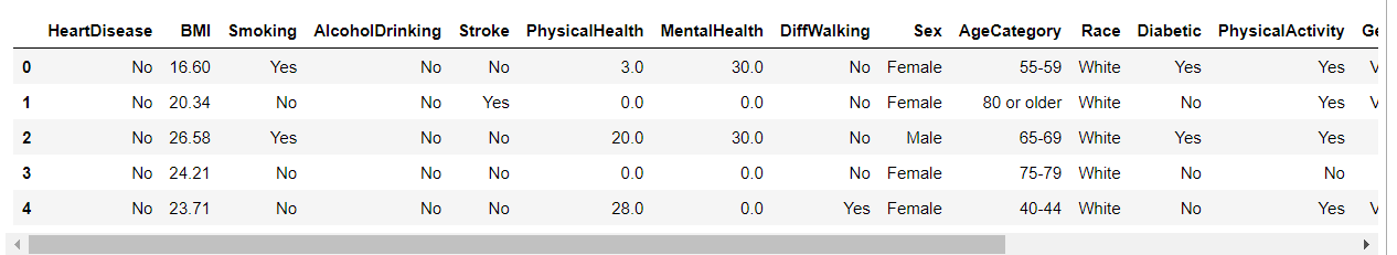
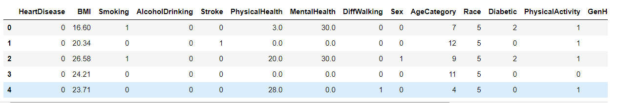
df.head()
The file is in the name heart_disease, and the above line of code uploads data from external sources. ‘read_csv’ enables us to read csv files. The code df. Head () displays the top 5 rows of the dataset as follows.
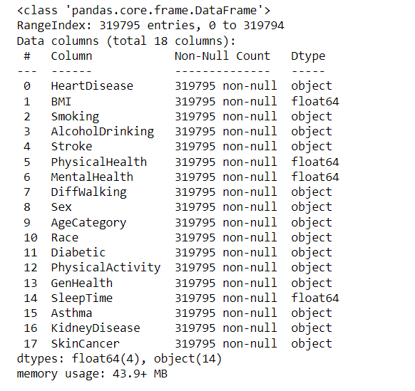
Next, we need to find the information in the dataset. This can be done by using the info() function. The information would comprise range index, data columns, non-null count, memory usage, and datatypes. The following are the line of code and the output.
df.info()
Next, we check for null values in the pandas dataframe with the help of the isnull() function. The function isnull().sum() displays the missing values in the dataset. The line of code and the output are
df.isnull().sum()Output
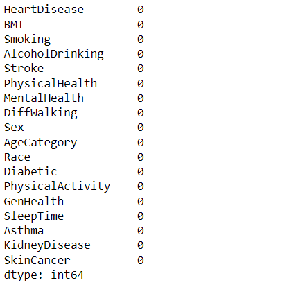
From the output, it can be seen that there are no missing values in the dataset. Next, we would like to get the data type of each column in the form of a series. The line of code and the output are as follows.
obj_list = df.select_dtypes(include='object').columns
obj_list
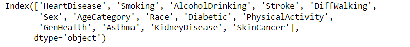
Here, we have created an object list including object datatype.
Next, we would encode target labels with values 0 and n-classes-1. This would transform the labels into the form of numbers that the machine can easily read. For this purpose, we would import the LabelEncoder module from sklearn.preprocessing library. Following are the lines of code and the outputs
from sklearn.preprocessing import LabelEncoder
le = LabelEncoder()
for obj in obj_list:
        df[obj] = le.fit_transform(df[obj].astype(str))
df.head()
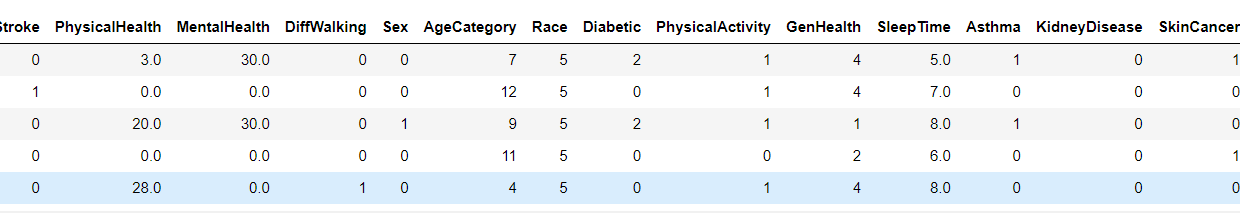
From the output, it can be seen that labels have been transformed into numeric forms. Next, we want to check the relationship between each parameter and the heart disease targeted. This will be achieved by using the correlation function. Correlation measures the strength of the relation between 2 datasets, with a positive correlation showing a strong dependency of one variable on the other and a negative correlation showing an inverse relationship. The range of correlation ranges between -1 and +1. The lines of code and the output are as follows
correlation=df.corr()
correlation
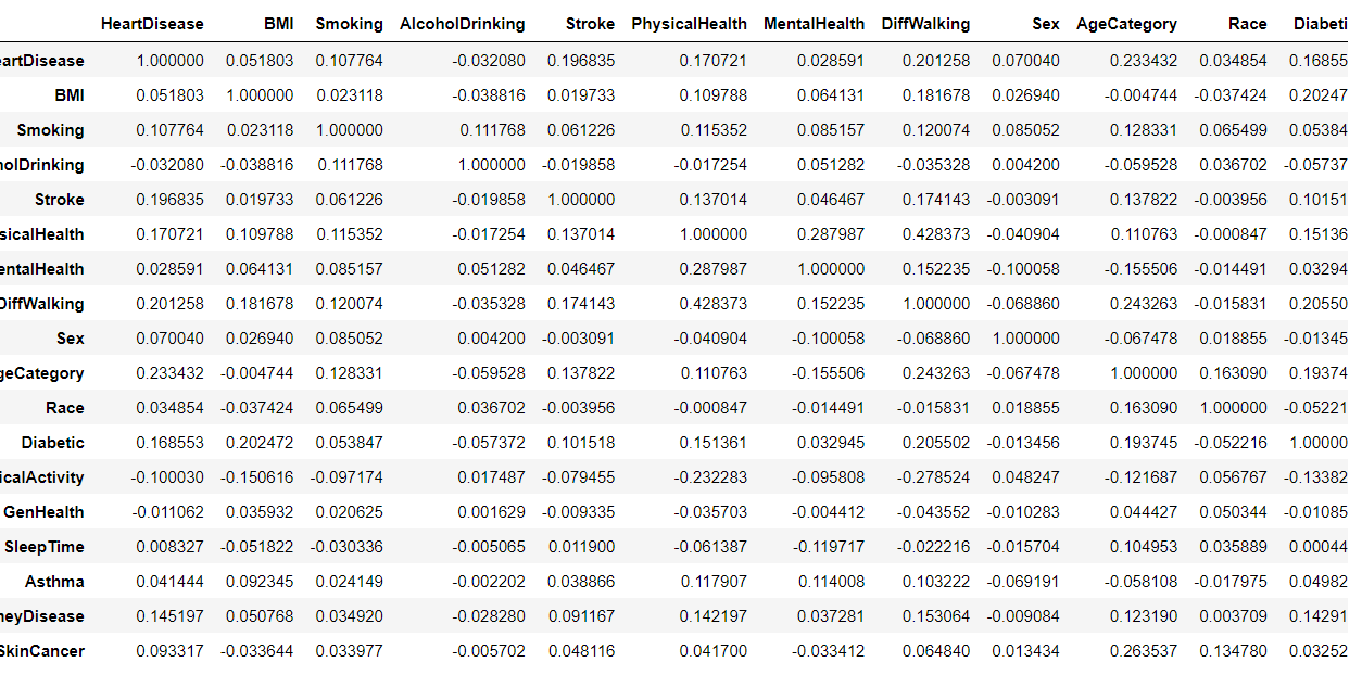
From the above output, let us analyze some variables concerning our target, i.e., Heart Disease. BMI=0.051803, smoking=0.107764, Alcohol drinking = -0.032080, Stroke = 0.196835, Physical Health = 0.170721, Mental Health = 0.028591, Age category = 0.233432, Diabetic = 0.168553, Physical activity = -0.100030, General Health = -0.011062, and Sleep time = 0.008327.
It can be seen that physical activity and general health are associated with reduced adverse cardiac outcomes; in contrast, stroke, diabetes, smoking, and physical health status are relatively positively associated with adverse cardiac outcomes.
Model Development
We shall proceed to label the inputs and the output. Here, ‘Disease’ is the target variable,e, and whether the individual concerned will have heart disease shall be determined based on the provided inputs. The first step of model development would be to perform a train-test split by importing the train_test_split method from the sklearn library. X would have independent variables, and y would have the target variable. 30% of the dataset would be the testing data. For a deterministic train-test split, random_state is set to an integer value. So, lines of code are
X = df.drop('HeartDisease', axis=1).values
y = df['HeartDisease'].values
from sklearn.model_selection import train_test_split
np.random.seed(41)
X_train, X_test, y_train, y_test = train_test_split(X, y, test_size=0.3)
The above line of code would split the data into train and test datasets to measure the model generalization and predict unseen data of the model. Now, we shall develop the model with the help of 2 different algorithms, viz. kNN, Logistic Regression, and Random Forest classifier.
KNN
kNN works by selecting the number k of the neighbors and calculating Euclidean distance. Then, the number of data points is counted in each category, and the new data points are assigned to that category. Let’s look at the lines of code and the respective output in the form of accuracy
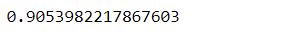
from sklearn.neighbors import KNeighborsClassifier
knn = KNeighborsClassifier().fit(X_train, y_train)
knn.score(X_test, y_test)
Logistic Regression
From sklearn.linear_model, we shall import the logistic regression module and then fit training data. Let’s look at the lines of code and the respective output in the form of accuracy.y
from sklearn.linear_model import LogisticRegression
np.random.seed(41)
lr = LogisticRegression().fit(X_train, y_train)
lr.score(X_test, y_test)

Random Forest Classifier
From sklearn.ensemble, we shall import the logistic random forest classifier module and then fit training data. Let’s look at the lines of code and the respective output in the form of accuracy.y
from sklearn.ensemble import RandomForestClassifier
np.random.seed(41)
rf = RandomForestClassifier().fit(X_train, y_train)
rf.score(X_test, y_test)

In all the above cases, we have used np.random.seed() to get the luckiest numbers for each run. Through accuracy score, we have evaluated the performance of various models.
Model Evaluation
Though we have evaluated the models with the help of an accuracy score, the confusion matrix would enable us further to understand the misclassification aspect of the model development process. The confusion matrix is depicted below
| Predicted: Yes | Predicted: No | Total | |
| Actual: Yes | a (T.P) | b (F.N) | a+b (Actual yes) |
| Actual: No | c (F.P) | d (T.N) | c+d (Actual No) |
| Total | a+c (Predicted yes) | b+d (Predicted No) | a+b+c+d |
| Here, T.P = True Positive, F.N = False Negative, F.P = False Positive, T.N = True Negative
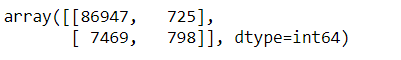
Confusion matrix through KNN, Logistic Regression, and Random Forest Classifier Logistic Regression |
from sklearn.metrics import confusion_matrix
prediction=lr.predict(X_test)
prediction
confusion_matrix=confusion_matrix(y_test,prediction)
confusion_matrix
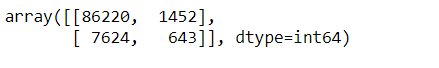
KNN
from sklearn.metrics import confusion_matrix
prediction=knn.predict(X_test)
prediction
confusion_matrix=confusion_matrix(y_test,prediction)
confusion_matrix
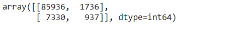
Random Forest Classifier
from sklearn.metrics import confusion_matrix
prediction=rf.predict(X_test)
prediction
confusion_matrix=confusion_matrix(y_test,prediction)
confusion_matrix
Conclusion
Among the classifiers, we can see that KNN had an accuracy of 90.53%, logistic regression had a precision of 91.45%, and random forest classifier had an accuracy rate of 90.55%. Further evaluation of the model entails generating the confusion matrix to understand the classification pattern. In the case of logistic regression, 87,745 out of 95,939 samples were correctly classified, whereas it is 86,863 for KNN and 86,873 for the random forest classifier. Though all the algorithms performed to the tune of more than 90 accuracy, logistic regression was the most accurate.
Key Takeaways
- KNN, logistic regression, and random forest classifiers can segregate individuals into high and low-risk categories with a high accuracy rate.
- A confusion matrix is a crucial tool to understand the misclassification aspect of the model.
- High blood pressure, high cholesterol, smoking, diabetic status, and physical activity are important factors that cause heart disease.
- Machine learning enables the detection of patterns from the data to predict the patient’s condition.
Frequently Asked Questions
Q1. Which algorithm is best for predicting heart disease?
A. Several algorithms like Random Forest, SVM, and Neural Networks perform well in predicting heart disease, each leveraging different features to achieve accurate results based on dataset characteristics.
Q2. How is machine learning useful in disease prediction?
A. Machine learning aids disease prediction by analyzing patient data to identify patterns, risk factors, and correlations, enabling early detection and personalized treatment plans, potentially saving lives.
Q3. What are the methodologies of heart disease prediction?
A. Heart disease prediction methodologies include risk assessment models, machine learning algorithms utilizing patient history, genetic predisposition, and lifestyle factors, empowering proactive intervention and preventive measures.
Q4. What is the role of AI in heart disease?
A. AI in heart disease augments diagnostics, analyzes vast medical data for accurate predictions, assists in risk stratification, and facilitates personalized treatment plans, revolutionizing healthcare by enhancing early detection and prognosis.
The media shown in this article is not owned by Analytics Vidhya and is used at the Author’s discretion.
I am a biotechnology graduate with experience in Administration, Research and Development, Information Technology & management, and Academics of more than 12 years. I have experience of working in organizations like Ranbaxy, Abbott India Limited, Drivz India, LIC, Chegg, Expertsmind, and Coronawhy.
Recognition:
1. Played major role in making a brand “Duphaston” worth “Rs 100 crores INR” in Abbott India Limited as Therapy Business Manager of Women’s health and gastro intestine team.
2. Won “best marketing skills” award in Abbott India Limited.
3. Came on the merit list of National IT aptitude test, 2010.
4. Represented my school in regional social science exhibition.
Courses and Trainings:
1. Took 54 hours training on vb.net in Niit, Guwahati.
2. Underwent training of 7 days on targeting and segmentation in Abbott India ltd, Lonavala.
3. Earned “Elite Certificate” from IIT-Madras on “Python for Data Science”.


what a good piece of knowledge. good article about heart health.
can i get this dataset
Great article. Is it possible to obtain this data? with all gratitude and appreciation