This article was published as a part of the Data Science Blogathon.
Introduction
We’ve all heard of the stock market, right? Stock is essentially a share in a specific company. The stock market is a risky game, but with the appropriate strategies and research, an investor can create generational wealth. This project is just a tiny fraction of analyzing stock market data with the help of Python since stock analysis includes both technical and fundamental analysis, which is a broad area.
This short python stock analysis of three significant stocks in the Indian stock market will point you in the correct direction for developing your data analysis and visualization skills, as well as assist you on the right path in the field.
Libraries Used
The libraries used in this project make data analysis and visualisation quite simple. These libraries can be downloaded by executing the pip command in the terminal:
pip install library_name
The libraries that are used are briefly described below:
| Library Name | Description |
| Pandas | To manipulate and analyze data |
| Matplotlib | For data visualization (Plot graphs) |
Data Set and Data Description
The data set I have used in this project has been downloaded from Kaggle (NIFTY-50 Stock Market Data (2000 – 2021)). You can head to this link and click the Download button.
 _ Kaggle - Brave 18-06-2022 13_47_58.png)
Once downloaded, extract the zip file.
This data set consists of a number of companies’ stock data from 2000-2021 including Adani Ports, Bajaj Finance, Wipro, Infosys, and many more. But for this project, we will be analyzing three Tata stocks – Tata Motors, Tata Steel, and Tata Consultancy Services (TCS).
The data in the data set consists of Date, Symbol, Prev Close, Open, High, Low, Last, Close, VWAP, Turnover, Trades, Deliverable Volume, and % Deliverable.
We will be utilizing the Date, Open, and Volume.
Data Analyzing and Exploring
Importing packages
import pandas as pd

import matplotlib.pyplot as plt
Importing Dataset
tata_motors=pd.read_csv("Stock_Data/TATAMOTORS.csv")
tata_steel=pd.read_csv("Stock_Data/TATASTEEL.csv")
tcs=pd.read_csv("Stock_Data/TCS.csv")
Viewing Data
import pandas as pd
tata_motors = pd.read_csv('TATAMOTORS.csv')
tata_steel = pd.read_csv('TATASTEEL.csv')
tcs = pd.read_csv('TCS.csv')

print(tata_motors.head())
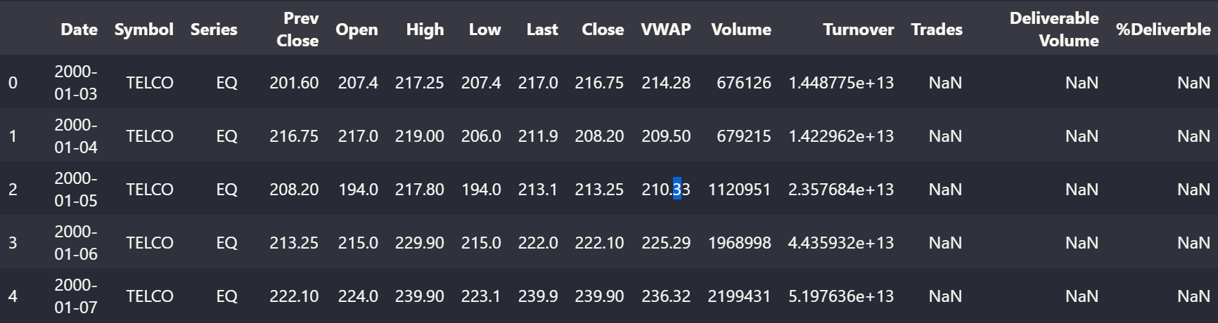
From the above table, we can view the first 5 rows of the Tata Motors dataset and get a brief overview of the data present.
You will see the results of the dataset for Tata Steel and TCS by executing the tata_steel.head() and tcs.head() functions respectively.
Checking Size of Data
tata_motors.shape
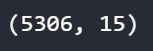
Here, we can see the size of the data set. 5306 represents a number of rows and 15 represents a number of columns.
After executing the tata_steel.shape and tcs.shape functions, you will see the size i.e the number of rows x columns of the Tata Steel and TCS dataset respectively.
Viewing Datatypes of all columns
tata_motors.info()
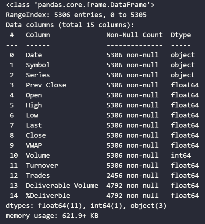
Here, we can notice the data type of “Date” is an ‘object’ in the Tata Motors dataset, hence we need to convert it into the ‘date’ datatype (Which we will do in the “Working on Data” section).
You will see similar results for the datatypes for Tata Steel and TCS datasets after executing the tata_steel.info() and tcs.info() functions respectively.
Checking for Null Values
tata_motors.isna().sum()
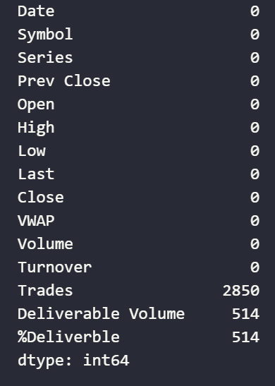
The columns Trades, “Deliverable”, “Volume” and “%Deliverable” have some NULL values present. We will drop these columns in the “Working on Data” section. These columns will not be used in our analysis.
You will see similar results for the datasets of Tata Steel and TCS after executing the tata_steel.isna().sum() and tcs.isna().sum() functions respectively.
Checking for Duplicate Values
tata_motors.duplicated().sum()

tata_steel.duplicated().sum()

tcs.duplicated().sum()
The output for each of the above codes comes as 0, which indicates there are no duplicate values present in the data set.
Description of Data in the Dataframe and rounding its values up to two decimal places
tata_motors.describe().round(2)
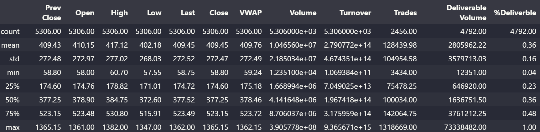
The describe function will show you statistical data such as the Count of nonnull values, Mean, Standard Deviation, etc of the data present in the dataset. The round(2) function rounds up the values up to two decimal places.
You will see the statistical data for the datasets of Tata Steel and TCS after executing the tata_steel.describe().round(2) and tcs.describe().round(2) respectively.
Working on Data
Converting the “Date” column dtype from object to date
tata_motors["Date"]=pd.to_datetime(tata_motors["Date"])
tata_steel["Date"]=pd.to_datetime(tata_steel["Date"])
tcs["Date"]=pd.to_datetime(tcs["Date"])
Once this code is executed, if you try executing the .info() function on any of the datasets, you will notice the datatype of the ‘Date’ column changed from ‘object’ to ‘datetime64[ns]’ for all 3 datasets.
Dropping columns Trades, Deliverable Volume, and %Deliverable
tata_motors=tata_motors.drop(['Trades','Deliverable Volume','%Deliverble'], axis=1)
tata_steel=tata_steel.drop(['Trades','Deliverable Volume','%Deliverble'], axis=1)
tcs=tcs.drop(['Trades','Deliverable Volume','%Deliverble'], axis=1)
Once this code is executed, if you try running the .head() or .tail() function on any of the datasets, you will notice all the 3 columns Trades, Deliverable Volume, and %Deliverable not present.
Adding 3 more new columns to each of the Dataset
tata_motors['Month']=tata_motors["Date"].dt.month

tata_motors['Year']=tata_motors["Date"].dt.year

tata_motors['Day']=tata_motors["Date"].dt.day


tata_steel['Month']=tata_steel["Date"].dt.month

tata_steel['Year']=tata_steel["Date"].dt.year

tata_steel['Day']=tata_steel["Date"].dt.day


tcs['Day']=tcs['Date'].dt.day

tcs['Year']=tcs['Date'].dt.year

tcs['Month']=tcs['Date'].dt.month
Once this code is executed, if you try running the .head() or .tail() function on any of the datasets, you will notice 3 new columns ‘Day’, ‘Month’ and ‘Year’ present. We will be using the ‘Day’ column for our analysis.
Comparing the Data
Price Comparision
plt.figure(figsize=(20,7))

plt.plot(tata_motors['Date'],tata_motors['Open'],color='blue',label='Tata Motors')

plt.plot(tata_steel['Date'],tata_steel['Open'],color='grey',label='Tata Steel')

plt.plot(tcs['Date'],tcs['Open'],color='orange',label='TCS')


plt.title("Relation between Tata Motors, Tata Steel and TCS Price")

plt.xlabel("Year")

plt.ylabel("Price")

plt.legend(title="")

plt.show()
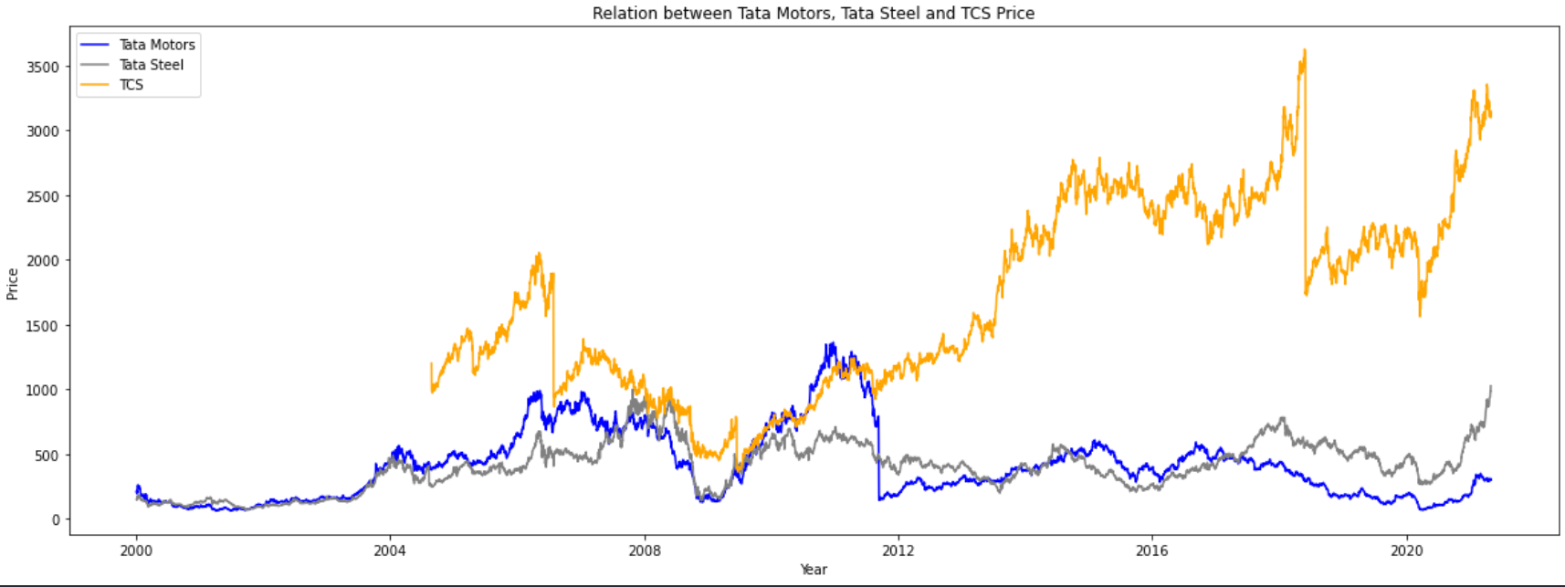
According to the graph above, the price of TCS has skyrocketed significantly higher than that of Tata Steel and Tata Motors. TCS’s pricing trajectory has been generally upward from its beginning, whereas Tata Steel and Tata Motors have been more on a consolidation trend.
Volume Comparision
plt.figure(figsize=(20,7))

plt.plot(tata_motors['Date'],tata_motors['Volume'],color='blue',label='Tata Motors')

plt.plot(tata_steel['Date'],tata_steel['Volume'],color='grey',label='Tata Steel')

plt.plot(tcs['Date'],tcs['Volume'],color='orange',label='TCS')


plt.title("Relation between Tata Motors, Tata Steel and TCS Volume")

plt.xlabel("Year")

plt.ylabel("Volume")

plt.legend(title="")

plt.show()
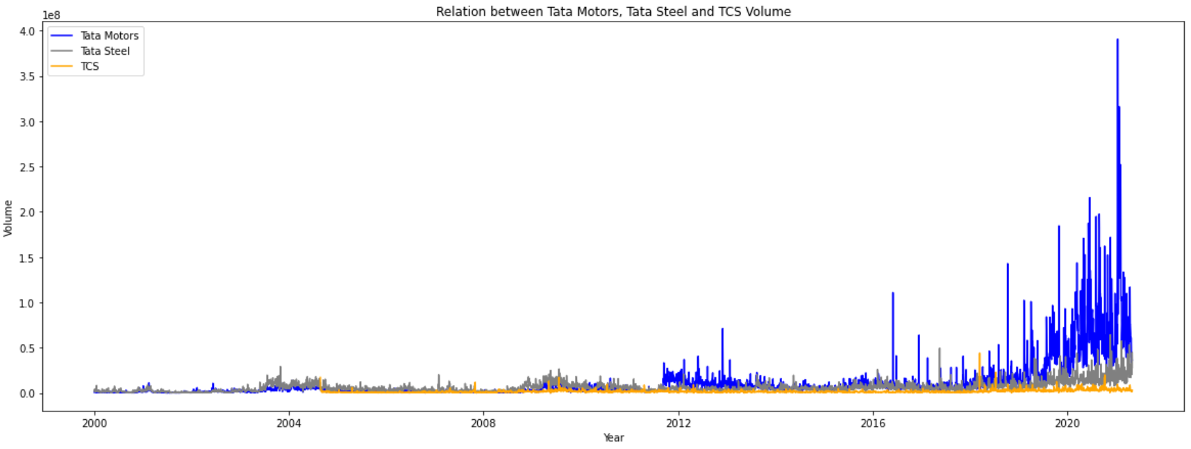
Though the price of TCS has risen more significantly as compared to Tata Steel and Tata Motors, we can notice from the above graph that TCS has the least volume signifying that the python stock analysis has been traded comparatively less as compared to Tata Steel and Tata Motors and is lesser liquid.
Tata Motors on the other hand has been traded the most signifying higher liquidity, and better order execution.
Return on Investment (ROI)
In this part, we will analyze the ROI of Tata Steel, Tata Motors, and TCS if we buy one share of each stock on the 30th of each month beginning from January 2000 for Tata Motors and Tata Steel and November 2004 for TCS.
Tata Motors ROI
sumTM=0 #total amount invested in Tata Motors
s1=0 #number of shares owned by Tata Motors
#calcuating total amount invested and number of shares owned in Tata Motors
for i in range(len(tata_motors)):
if tata_motors.loc[i,'Day']==30:
sumTM+=tata_motors.loc[i,'Open']
s1+=1
#displaying basic results
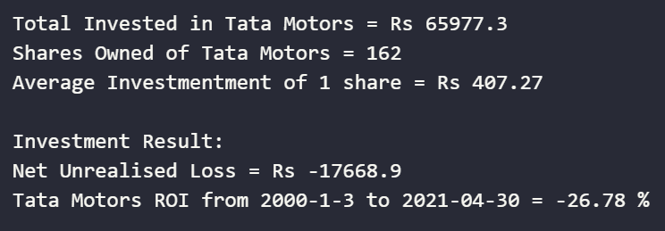
print("Total Invested in Tata Motors = Rs",round(sumTM,2))
print("Shares Owned of Tata Motors =",s1)
print("Average Investmentment of 1 share = Rs",round((sumTM/s1),2))
tm_end=298.2 #last open price of Tata Motors on 2021-04-30
#obtained by looking at the data or can be seen after executing tata_motors.tail()
#calculating investment results
result1=round((tm_end*s1)-sumTM,2)
roiTM=round((result1/sumTM)*100,2)
#displaying investment results
print("nInvestment Result:")
if result1<0:
print("Net Unrealised Loss = Rs",result1)
else:
print("Net Unrealised Profit = Rs",result1)
print("Tata Motors ROI from 2000-1-3 to 2021-04-30 =",roiTM,"%")
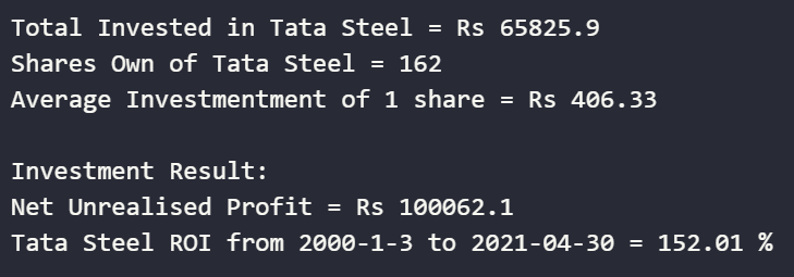
Tata Steel ROI
sumTS=0 #total amount invested in Tata Steel

s2=0 #number of shares owned by Tata Steel
#calcuating total amount invested and number of shares owned in Tata Steel

for i in range(len(tata_steel)):

    if tata_steel.loc[i,'Day']==30:

        sumTS+=tata_steel.loc[i,'Open']

        s2+=1


#displaying basic results

print("Total Invested in Tata Steel = Rs",round(sumTS,2))

print("Shares Own of Tata Steel =",s2)

print("Average Investmentment of 1 share = Rs",round((sumTS/s2),2))


ts_end=1024 #last open price of Tata Steel on 2021-04-30

#obtained by looking at the data or can be seen after executed tata_steel.tail()
#calculating investment results

result2=round((ts_end*s2)-sumTS,2)

roiTS=round((result2/sumTS)*100,2)


#displaying investment results

print("nInvestment Result:")


if result2<0:

    print("Net Unrealised Loss = Rs",result2)

else:

    print("Net Unrealised Profit = Rs",result2)
print("Tata Steel ROI from 2000-1-3 to 2021-04-30 =",roiTS,"%")
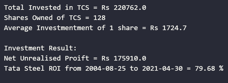
TCS ROI
sumTCS=0 #total amount invested in TCS

s3=0 #number shares owned of TCS


#calcuating total amount invested and number of shares owned in TCS

for i in range(len(tcs)):

    if tcs.loc[i,'Day']==30:

        sumTCS+=tcs.loc[i,'Open']

        s3+=1


#displaying basic results

print("Total Invested in TCS = Rs",round(sumTCS,2))

print("Shares Owned of TCS =",s3)

print("Average Investmentment of 1 share = Rs",round((sumTCS/s3),2))


tcs_end=3099 #last open price of TCS on 2021-04-30

#obtained by looking at the data or can be seen after executed tcs.tail()


#calculating investment results

result3=round((tcs_end*s3)-sumTCS,2)

roiTCS=round((result3/sumTCS)*100,2)


#displaying investment results

print("nInvestment Result:")


if result3<0:

    print("Net Unrealised Loss = Rs",result3)

else:

    print("Net Unrealised Proift = Rs",result3)


print("Tata Steel ROI from 2004-08-25 to 2021-04-30 =",roiTCS,"%")
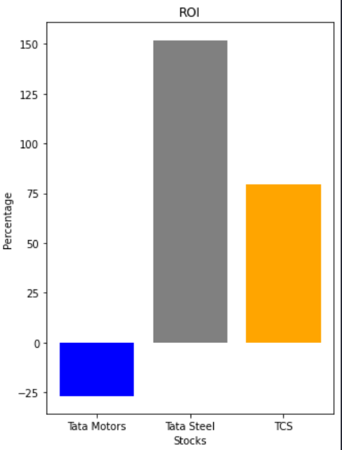
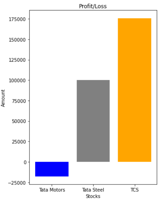
From the above results, we can conclude that Tata Steel’s ROI is significantly larger than that of Tata Motors and TCS. TCS on the other hand, has made the greatest profit.
Investment Results (Graphically)
Plotting ROI on Bar Graph
plt.figure(figsize=(5,7))

stock=['Tata Motors','Tata Steel','TCS']

ROI=[roiTM,roiTS,roiTCS]

col=['Blue','Grey','Orange']


plt.bar(stock,ROI,color=col)


plt.title("ROI")

plt.xlabel("Stocks")

plt.ylabel("Percentage")
Plotting Profit/Loss Amount on Bar Graph
plt.figure(figsize=(5,7))

stock=['Tata Motors','Tata Steel','TCS']

amt=[result1,result2,result3]

col=['Blue','Grey','Orange']


plt.bar(stock,amt,color=col)


plt.title("Profit/Loss")

plt.xlabel("Stocks")

plt.ylabel("Amount")
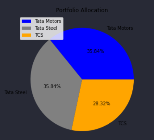
Portfolio Allocation
Displaying Number of shares owned.
plt.figure(figsize=(5,7))

stock=['Tata Motors','Tata Steel','TCS']

shares=[s1,s2,s3]

col=['Blue','Grey','Orange']


plt.pie(shares,labels=stock,autopct="%1.2f%%",colors=col)

plt.legend(title="",loc="upper left")

plt.title("Portfolio Allocation")
Conclusion
This is NOT FINANCIAL ADVICE, and all work done in this project is for educational purposes only. This analysis depicts a stock’s long-term performance and shows the potential of SIP in the long run.
Feel free to connect with me. Hope you liked my article on python stock analysis. Thank you for your time.
The media shown in this article is not owned by Analytics Vidhya and is used at the Author’s discretion.
A crypto research analyst, algorithmic trader who is passionate about cryptocurrency, finance, investing and data analytics.
In this blog, I will be mainly focusing on how to use python programming language to derive meaningful insights from datasets in order educate and develop various investing strategies for assets.
In addition, I will be uploading "how to" guides on various decentralized applications running on a number of blockchains and "Top 5" guides. Furthermore, research articles on blockchain projects will be a part of the content.


Great explanation! before I read this I understood nothing but now I feel like a total pro. jeez!