End-to-End Project on SMS/Email Spam Detection using Naive Bayes

This article was published as a part of the Data Science Blogathon.

Introduction to Naive Bayes

With the increase in online consumption of products and services, consumers are facing a huge problem of abundance of spam messages in their inboxes which are either promotional-based or fraudulent. But due to this the messages/Email which is of much importance are squashed under the spam messages.

In this article, we are going to create an SMS spam detection model which will help you to find whether an SMS is a spam or not using Naive Bayes and Natural Language Processing(NLP).

Gathering and Loading Data

For this particular project, we will be using the dataset available on the Kaggle SMS Spam Collection Dataset which has a set of SMS-tagged messages in English that have been classified as being ham (‘legitimate’) and spam. Each line holds one message. Two columns make up each line:v1 carries the label such as (spam or ham) and v2 contains the actual content.

Output

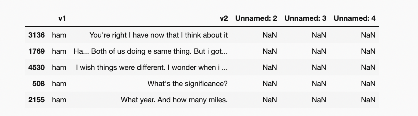
output of dataset

Now let’s start working on the dataset and make some amazing visualisations and conclusions.

Data Cleaning

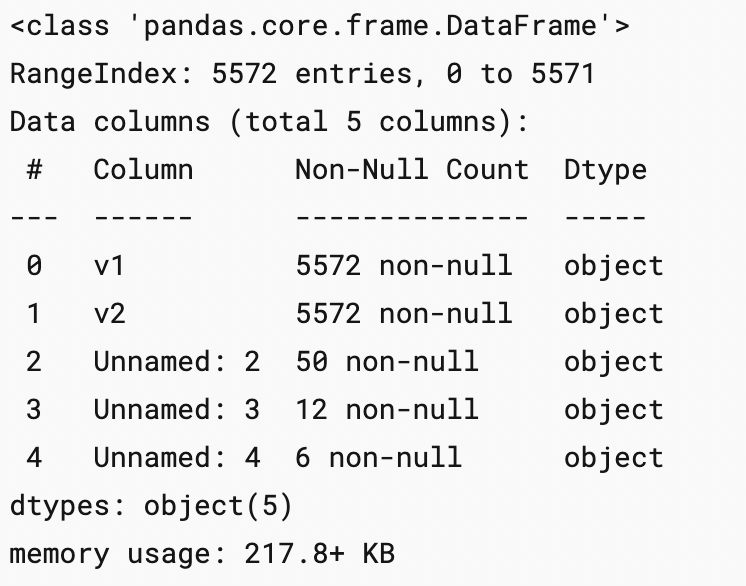
df.info()

Output

df.drop(columns=['Unnamed: 2','Unnamed: 3','Unnamed: 4'],inplace= True)
df.sample(5)

df.rename(columns={'v1':'message_type', 'v2':'message'},inplace=True)

df.sample(5)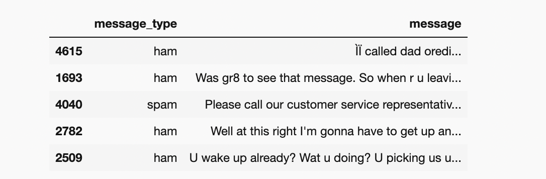

 As this is a classification problem we want the “message_type” to be binary classified i.e, 0 or 1 so for this purpose we use label encoder.

from sklearn.preprocessing import LabelEncoder
encoder =LabelEncoder()

df['message_type']=encoder.fit_transform(df['message_type'])
df['message_type'].sample(5)

df[df['message_type']==1]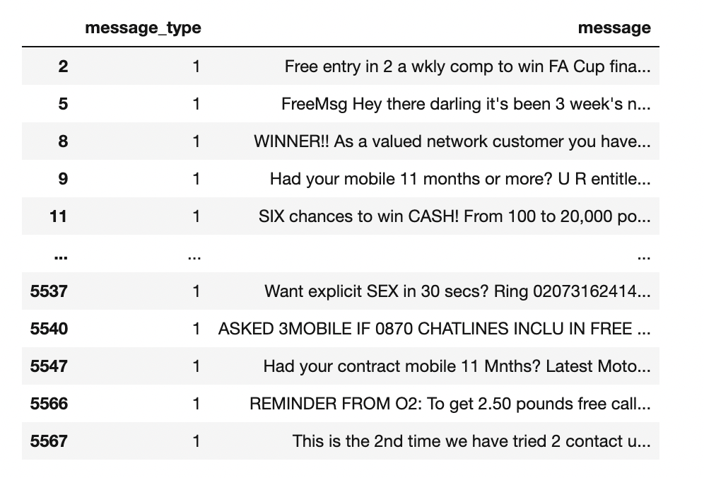

Now let’s check for the missing values

df.isnull().sum()
df.duplicated().sum()

There are 403 duplicated values and we have to remove them

df= df.drop_duplicates()

Exploratory Data Analysis

Let’s visualise the classification problem to get a better understanding of the data.

import seaborn as sns
import matplotlib.pyplot as plt

df['message_type'].value_counts()

plt.pie(df['message_type'].value_counts(),labels=[' not spam','spam'],autopct='%0.2f')
plt.show()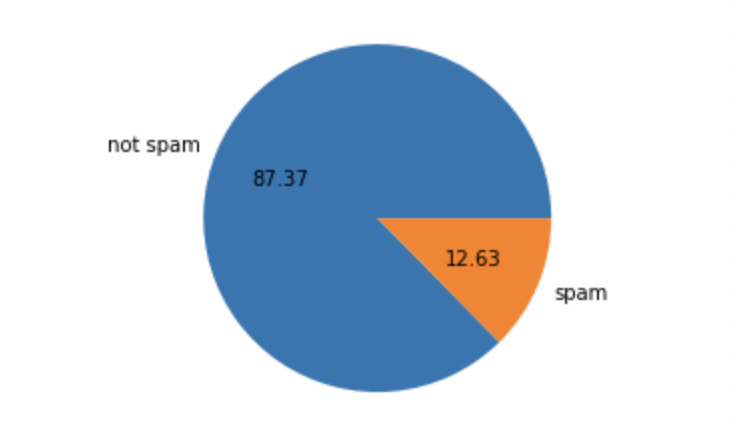

This is an imbalanced data

Now let’s find out :

• No. of characters in the data
• No. of words in the data
• No. of sentences in the data

and form 3 new columns in the data depicting the no. of character, words and sentences.

For a number of characters :

#natural language tool kit
import nltk
nltk.download('punkt')

df['num_characters']=df['message'].apply(len)
df.head()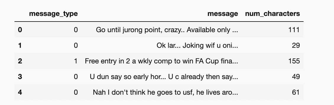

For a number of words :

from nltk.tokenize import word_tokenize
df['message'].apply(lambda x: nltk.word_tokenize(x))

df['num_words']=df['message'].apply(lambda x:len(nltk.word_tokenize(x)))
df.sample(5)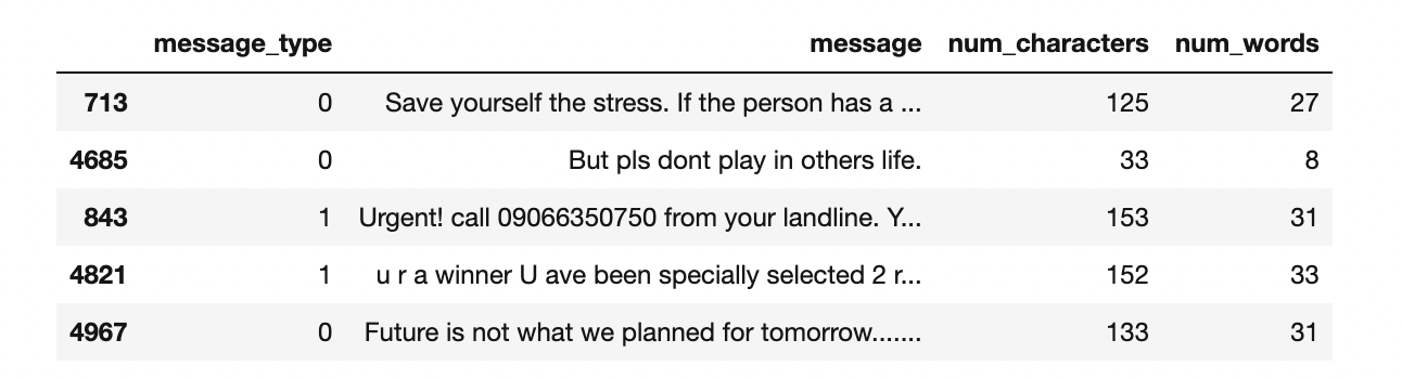

For a number of sentences :

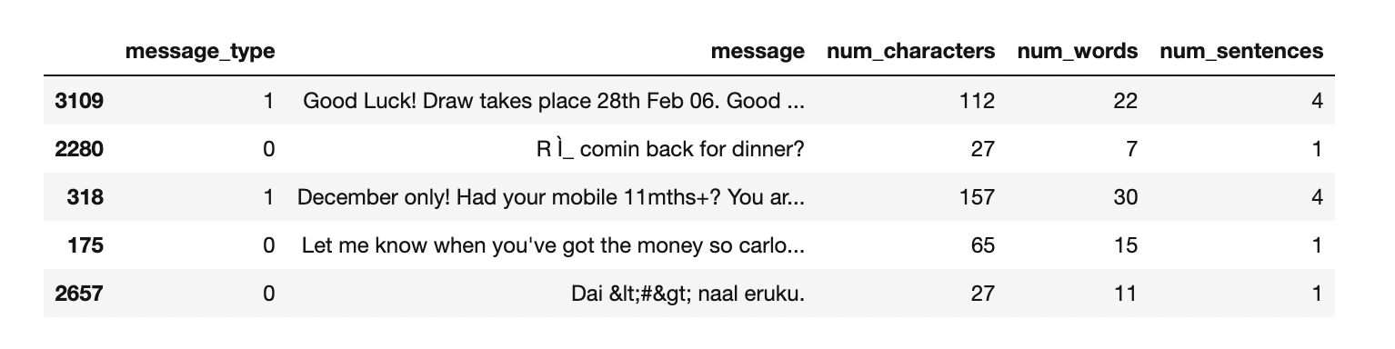
df['num_sentences']=df['message'].apply(lambda x: len(nltk.sent_tokenize(x)))

For ‘Ham’ messages:

df[df['message_type']==0][['num_characters','num_words','num_sentences']].describe()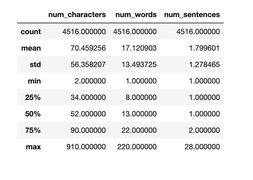

For ‘Spam’ messages:

df[df['message_type']==1][['num_characters','num_words','num_sentences']].describe()

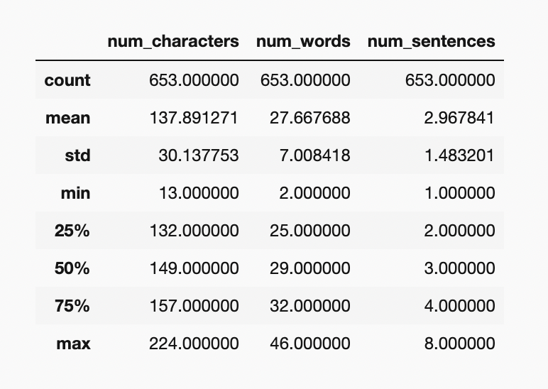
 We can clearly see the spam messages are quite longer than the ham messages.

#for characters
plt.figure(figsize=(12,6))
sns.histplot(df[df['message_type']==0]['num_characters'],color='green')
sns.histplot(df[df['message_type']==1]['num_characters'],color = 'red')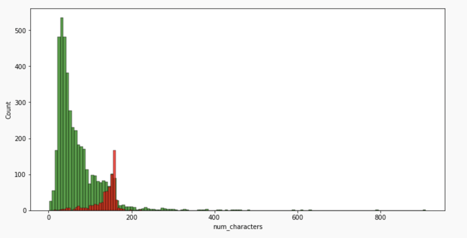

#for words
plt.figure(figsize=(12,6))
sns.histplot(df[df['message_type']==0]['num_words'],color='green')
sns.histplot(df[df['message_type']==1]['num_words'],color='red')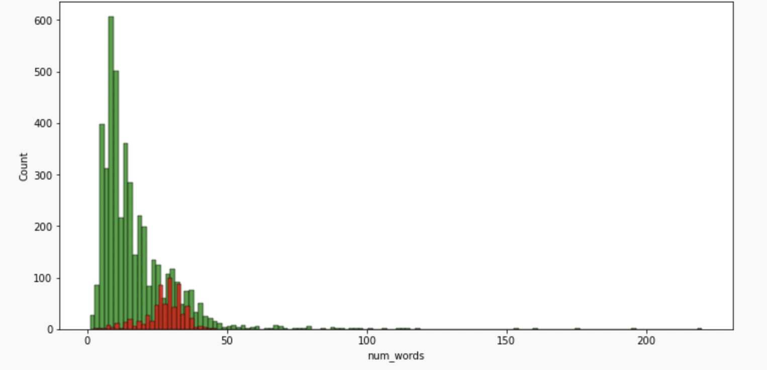

#plotting a heatmap for the correlation
sns.heatmap(df.corr(),annot=True)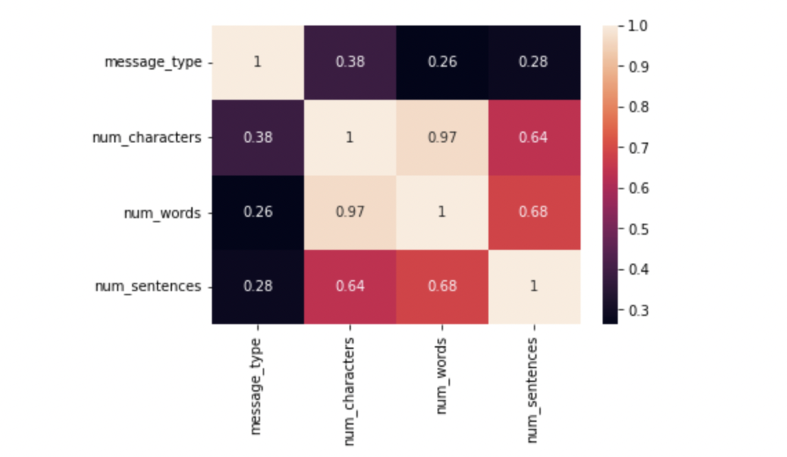

As we see multicollinearity here, we cannot use all three columns instead we shall use only one and that should be num_characters has it has highest correlation with message_type.

Data Preprocessing

3.1 LowerCase

3.2 Tokenisation

3.3 Removing special characters

3.4 Removing stop words and punctuation

3.5 Stemming — lemmatisation

def text_transform(message):
    message=message.lower() #change to lowercase
    message=nltk.word_tokenize(message)

    y=[] 
    for i in message:
        if i.isalnum():
            y.append(i)

        y.clear()

    
    #for checking punctuations and stopwords
    for i in message:
        if i not in stopwords.words('english') and i not in string.punctuation:
            y.append(i)
    message=y[:]
    y.clear()
    
    #now stemming function
    for i in message:
        y.append(ps.stem(i))
    
    #return y  --> returns as list
    return " ".join(y)

# Removing stop words and punctuations
nltk.download('stopwords')
from nltk.corpus import stopwords
stopwords.words('english')
len(stopwords.words('english')) 

#now for punctuation
import string
string.punctuation

# stemming
from nltk.stem.porter import PorterStemmer
ps =PorterStemmer()

Now let’s apply the text_transform function to all the messages in the dataset.

df['transformed_msg']=df['message'].apply(text_transform)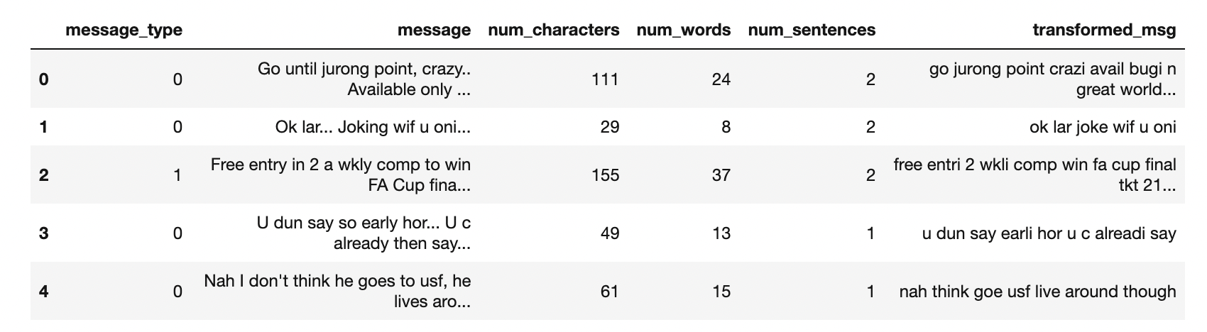

To get a clear idea about the most frequent words used we make a  word cloud.

from wordcloud import WordCloud
wc=WordCloud(width=500,height=500,min_font_size=10,background_color='white')

For Spam:

spam_wc=wc.generate(df[df['message_type']==1]['transformed_msg'].str.cat(sep=""))

plt.figure(figsize=(18,12))
plt.imshow(spam_wc)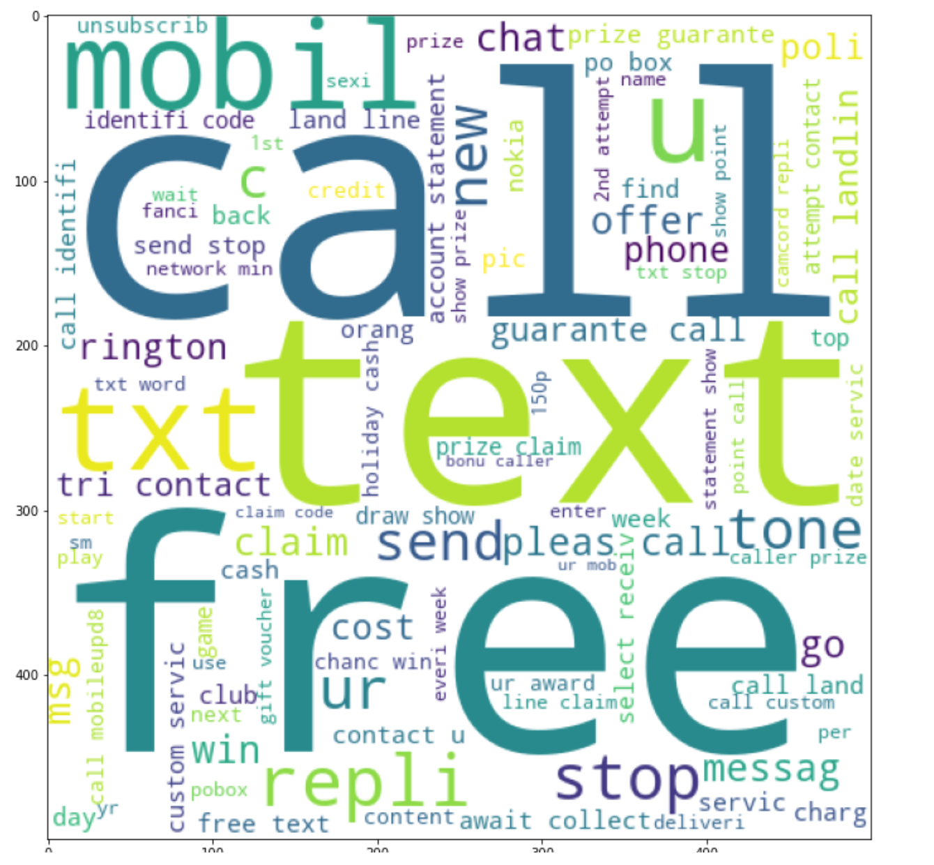

For Ham:

ham_wc=wc.generate(df[df['message_type']==0]['transformed_msg'].str.cat(sep=""))

plt.figure(figsize=(18,12))

plt.imshow(ham_wc)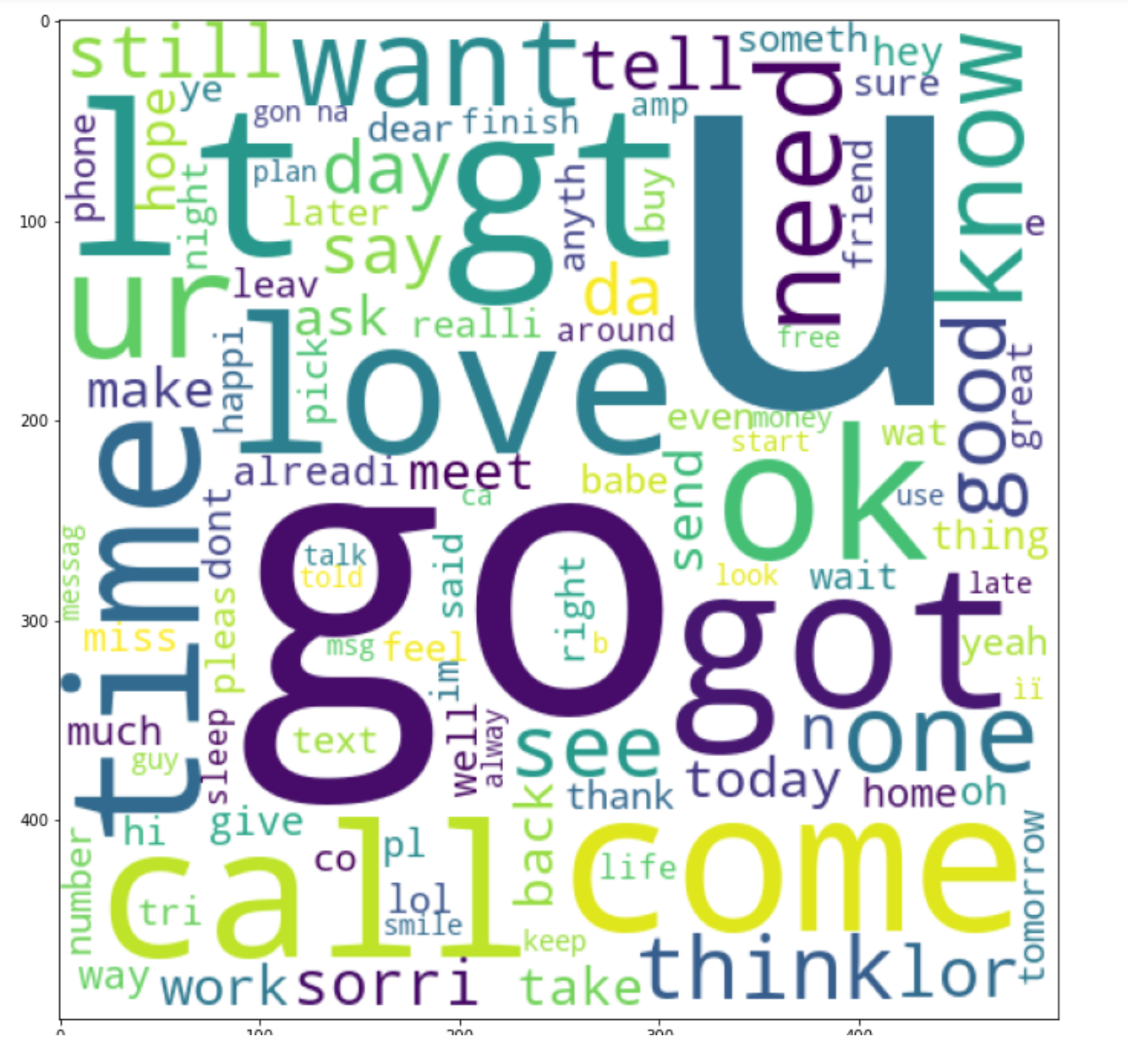

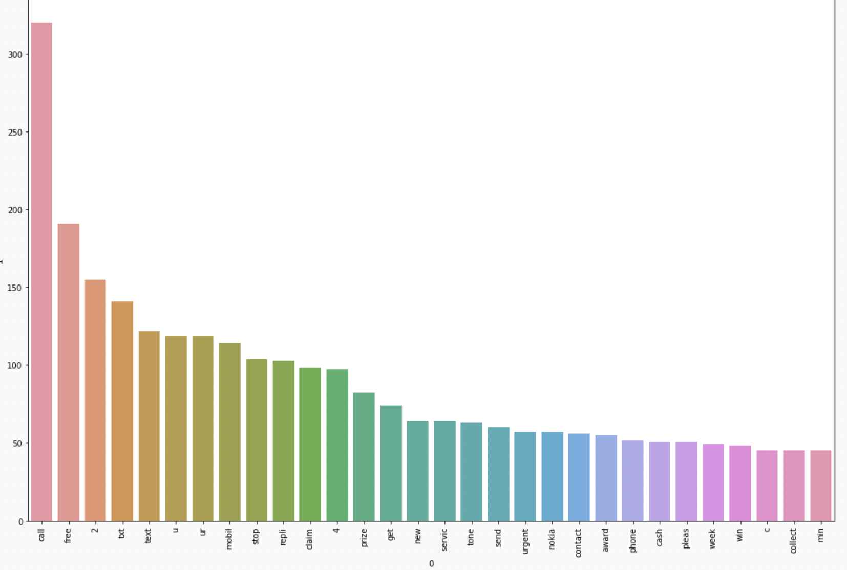
To simplify what is drawn inside the WordClouds we will find out the top 30 words used in both ham as well as spam messages.

spam_corpus=[]
for msg in df[df['message_type']==1]['transformed_msg'].tolist():
    for word in msg.split():
        spam_corpus.append(word)
from collections import Counter
Counter(spam_corpus)
Counter(spam_corpus).most_common(30)
plt.figure(figsize=(18,12))
sns.barplot(pd.DataFrame(Counter(spam_corpus).most_common(30))[0],pd.DataFrame(Counter(spam_corpus).most_common(30))[1])
plt.xticks(rotation='vertical')
plt.show()

Building a Model using Naive Bayes

As it is known that on Textual Data Naive Bayes Algorithm works the best hence we will use it but along the way also compare it with different algorithms

Input is categorical Output is Numerical.

But as we know in the Naive Bayes algorithm the input columns should be numerical so we have to convert (VECTORIZE) the column.

How to vectorize:

• Bag of Words
• TFIDF
• Word2vec

After trying out different techniques, I came to the conclusion that TFIDF vectorization gives the best accuracy and precision score so we will be using it.

from sklearn.feature_extraction.text import TfidfVectorizer
tfidf= TfidfVectorizer(max_features=3000) 
X=tfidf.fit_transform(df['transformed_msg']).toarray()
y=df['message_type'].values
from sklearn.model_selection import train_test_split
X_train,X_test,y_train,y_test = train_test_split(X,y,test_size=0.2,random_state=2)

from sklearn.naive_bayes import GaussianNB
from sklearn.naive_bayes import BernoulliNB
from sklearn.naive_bayes import MultinomialNB
from sklearn.metrics import accuracy_score
from sklearn.metrics import confusion_matrix
from sklearn.metrics import precision_score

gnb = GaussianNB()
bnb = BernoulliNB()
mnb = MultinomialNB()

Now find out the Accuracy score, confusion Matrix and Precision Score of all 3 types of Naive Bayes:

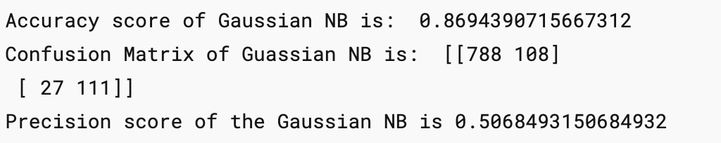
gnb.fit(X_train,y_train)
y_pred1= gnb.predict(X_test)
print('Accuracy score of Gaussian NB is: ',accuracy_score(y_test,y_pred1))
print('Confusion Matrix of Guassian NB is: ',confusion_matrix(y_test,y_pred1))
print('Precision score of the Gaussian NB is',precision_score(y_test,y_pred1))

mnb.fit(X_train,y_train)
y_pred2=mnb.predict(X_test)
print('Accuracy score of Multinomial NB is: ',accuracy_score(y_test,y_pred2))
print('Confusion Matrix of Multinomial NB is: ',confusion_matrix(y_test,y_pred2))
print('Precision score of the Multinomial NB is',precision_score(y_test,y_pred2))

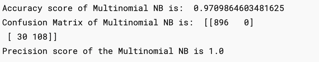
Here the precision comes out to be 1 which proves very good for our model as there will be no “FALSE POSITIVES”

bnb.fit(X_train,y_train)
y_pred3=bnb.predict(X_test)
print('Accuracy score of Bernoulli NB is: ',accuracy_score(y_test,y_pred3))
print('Confusion Matrix of Bernoulli NB is: ',confusion_matrix(y_test,y_pred3))
print('Precision score of the Bernoulli NB is',precision_score(y_test,y_pred3))

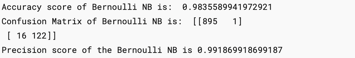
Hence we finalise the Model with MNB(Multinomial Naive Bayes) and TFIDF Vectorization.

Improving the Model

Change the max_feature parameter in TFIDF.

temp_df = pd.DataFrame({'Algorithm':clfs.keys(),'Accuracy_max_ft_3000':accuracy_scores,'Precision_max_ft_3000':precision_scores}).sort_values('Precision_max_ft_3000',ascending=False)

temp_df = pd.DataFrame({'Algorithm':clfs.keys(),'Accuracy_scaling':accuracy_scores,'Precision_scaling':precision_scores}).sort_values('Precision_scaling',ascending=False)

new_df = performance_df.merge(temp_df,on='Algorithm')

new_df_scaled = new_df.merge(temp_df,on='Algorithm')

temp_df = pd.DataFrame({'Algorithm':clfs.keys(),'Accuracy_num_chars':accuracy_scores,'Precision_num_chars':precision_scores}).sort_values('Precision_num_chars',ascending=False)

new_df_scaled.merge(temp_df,on='Algorithm')

After a lot of experiments and improvement, we have trained our model to get an Accuracy score of 97% and a precision Score of 100%.

Building a Website

import pickle
pickle.dump(tfidf,open('vectorizer.pkl','wb'))
pickle.dump(mnb,open('model.pkl','wb'))

2 files will be formed named “model.pkl” and “vectorizer.pkl”.

Open your IDE and create your own virtual environment. Install all the dependencies required using pip or conda. We will be building our website using streamlit so make sure that you download it too.

After the setup is ready make a file by “app.py”.

import streamlit as st
import pickle
import string
from nltk.corpus import stopwords
import nltk
from nltk.stem.porter import PorterStemmer
ps = PorterStemmer()
def transform_text(text):
    text = text.lower()
    text = nltk.word_tokenize(text)
    y = []
    for i in text:
        if i.isalnum():
            y.append(i)
    text = y[:]
    y.clear()
    for i in text:
        if i not in stopwords.words('english') and i not in string.punctuation:
            y.append(i)
    text = y[:]
    y.clear()
    for i in text:
        y.append(ps.stem(i))
    return " ".join(y)
tfidf = pickle.load(open('vectorizer.pkl','rb'))
model = pickle.load(open('model.pkl','rb'))
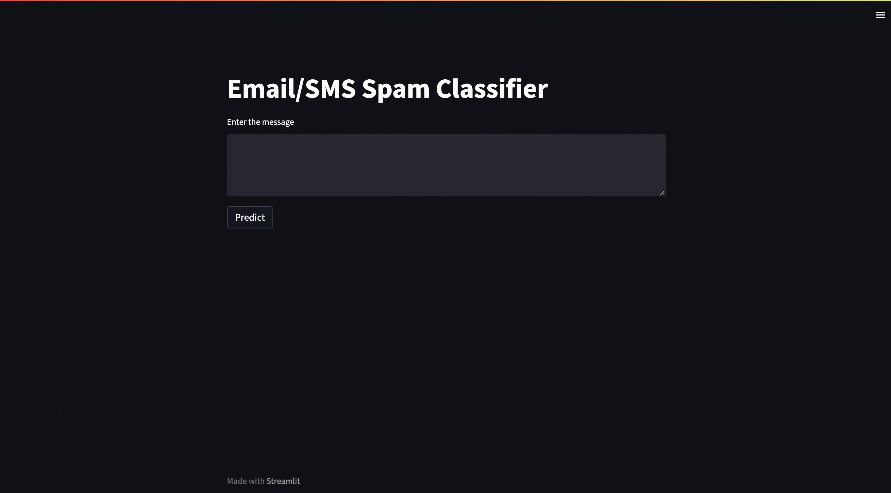
st.title("Email/SMS Spam Classifier")
input_sms = st.text_area("Enter the message")
if st.button('Predict'):
    # 1. preprocess
    transformed_sms = transform_text(input_sms)
    # 2. vectorize
    vector_input = tfidf.transform([transformed_sms])
    # 3. predict
    result = model.predict(vector_input)[0]
    # 4. Display
    if result == 1:
        st.header("Spam")
    else:
        st.header("Not Spam")

Now run the command to run the website on localhost:

streamlit run app.py

Deployment on Heroku

Deployment on Heroku is pretty straightforward;

Login to the Heroku website and create a new app.

Install the Heroku CLI and follow the given steps:

$ heroku login

$ cd my-project/
$ git init
$ heroku git:remote -a arcane-bayou-70408

Deploy your application

$ git add .
$ git commit -am "make it better"
$ git push heroku master

Your Website is up and running!!!

Heroku Deployment additional reference: https://devcenter.heroku.com/articles/git

Hurray! and now you have successfully completed an end-to-end machine learning project using the Naive Bayes Algorithm and Natural Language Processing.

You can check out my complete deployed project on: https://sms-spam-check.herokuapp.com/

and the source code is available in my Github profile:https://github.com/RiyaParikh0112/sms-spam-check

Conclusion on Naive Bayes

In this end-to-end guide we have learned how to approach a problem statement, and gather useful conclusions from the data using Data preprocessing, Data Visualisation which will help you build a good Machine Learning Model.

In order to solve this classification problem we used the Naive Bayes Algorithm and in particular, the Multinomial Naive Bayes algorithm as it was having the highest precision score (i.e least False Positives) and for the vectorization technique, we used TFIDF.

TF-IDF is an information retrieval technique that weighs a term’s frequency (TF) and its inverse document frequency (IDF). Each word or term that occurs in the text has its respective TF and IDF score.

The model was further improved using hyperparameter tuning in “max_features”.The following techniques helped us understand how to create a text classification model and make a .pkl file to use over networks. This guide provides an overview of using different techniques to classify a text message as “spam” or “not”.

You may probably already envision all the incredible potential and applications of this new information. This application may be included in chatbots, HR applications, and other systems. The possibilities are endless.

The media shown in this article is not owned by Analytics Vidhya and is used at the Author’s discretion.