Introduction to Tree Methods in MLIB

This article was published as a part of the Data Science Blogathon.

Introduction to MLIB

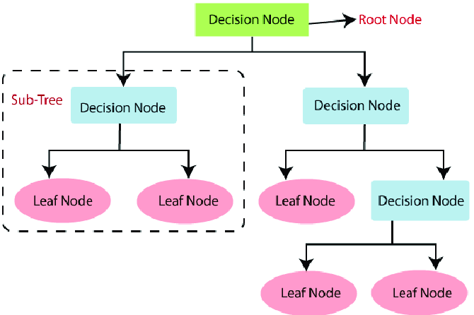
Tree methods are one of the most efficient ways of handling both the classification and the regression problems. There are ample methods available to choose from like Decision Tree, Random Forest, and Gradient Boosting. In this article, we will use the official dataset provided by Spark (perfectly cleaned and ready to use) so that we won’t be focussing much on data preprocessing and more on the model development and evaluating process.

This way, we can go through each tree algorithm in a detailed and descriptive way. So without wasting more time in story building let’s get our hands on building tree models using PySpark’s MLIB.

Installing PySpark

Before using PySpark’s methods, libraries, and utilities one will have to install the pyspark which is quite a straightforward step, we just have to use a simple command i.e. pip install pyspark.

Note: In the below cell note I used “!” before the command which denotes that it is the “Jupiter” notebook cell if one is using the command line then an exclamation sign is not required.

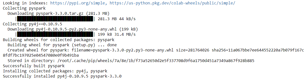
!pip install pyspark

Output:

Importing Required PySpark Libraries

Let’s start by importing the libraries as per the initial requirements we might end up importing more libraries as we move on with more functionalities meanwhile let’s get started with the first round of modules.

from pyspark.ml import Pipeline
from pyspark.ml.classification import RandomForestClassifier
from pyspark.ml.evaluation import MulticlassClassificationEvaluator

So we have imported mainly three libraries for now and they are Pipeline, RandomForestClassifier and MulticlassClassificationEvaluator let’s get a brief introduction for all three of them.

1. RandomForestClassifier: As the name denotes it is the Random forest algorithm for the classification problems.
2. Pipeline: This module helps us to maintain the proper workflow of the machine learning process and staging each step for hassle-free load balancing.
3. MulticlassClassificationEvaluator: This is the model evaluation metric more specifically for multi-class classification.

from pyspark.sql import SparkSession

spark = SparkSession.builder.appName('random_forest_intro').getOrCreate()
spark

Output:

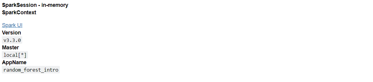
Inference: In the above set of codes we imported the SparkSession module and then we created the Spark object which is kind of the “must-todo” step for accessing and utilizing all the PySpark’s methods, and libraries and modules.

data_tree = spark.read.format("libsvm").load("sample_libsvm_data.txt")

Inference: So now we are loading that official dataset from the spark GitHub repository. Note that this one is not in the traditional CSV format instead of in lib-SVM format hence we will load it in that way only.

data_tree.show()

Output:

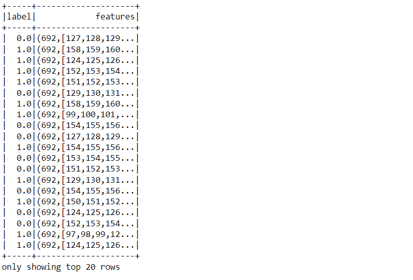
Inference: Here is the sneak peek of the dataset on which we will be working to apply tree algorithms one needs to notice that it is already preprocessed and cleaned just the way PySpark wants it to be and we don’t even have to use the VectorAssembler object because that task is also done.

data_tree.printSchema()

Output:

root
 |-- label: double (nullable = true)
 |-- features: vector (nullable = true)

Inference: As discussed earlier that we have preprocessed data hence one is the features column (Vector type) and the label column i.e. target column.

data_tree.head(5)

Inference: There is one more way to have a look into the dataset and this one is quite similar to pandas i.e. the head() method which not only will return the name and type of the columns but also the values of each are holding.

Train-Test split

This phase of the machine learning cycle is also known as splitting the dataset phase where we will break down the dataset into training and testing sets so that we can train the model on the training set and test the same on the testing set.

(trainingSet, testSet) = data_tree.randomSplit([0.7, 0.3])

Inference: RandomSplit() is the method that is responsible to divide the dataset into training and testing sets and from the parameter values we can stimulate that there is 70% of training data and 30% of testing data.

Now we will train the random forest model (here classifier) for that firstly the random forest object needs to be created by passing in the relevant parameter.

random_forest = RandomForestClassifier(labelCol="label", featuresCol="features", numTrees=20)

Inference: While creating the Random forest classifier we are passing the label column that is our target and the features column (collectively all the features) and as it is a random forest classifier so we have to specify the total number of trees as 20.

model_rf = random_forest.fit(trainingSet)

Inference: Now to train the model we use the fit() method by passing the set of training data as the parameter to that function and don’t forget to use the random forest object for calling it.

predictions = model_rf.transform(testSet)

Inference: Here comes the stage where we will make predictions using the evaluation method of the MLIB library and make sure to evaluate the model on testing data as then only the purpose of using it will be fulfilled.

predictions.printSchema()

Output:

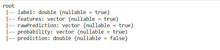
Inference: Let’s look at what the prediction DataFrame holds. So from the above output, we can see that there are 5 columns:

1. Label: This is the target column.
2. features: All the features/dependent columns in the form of vector
3. rawPrediction: This column will be very handy in the case of the GBT classifier
4. Probability: It holds the probability of how much are the chances that the predictions are correct.
5. Predictions: Predicted values by the model during evaluation.

predictions.select("prediction", "label", "features").show(5)

Output:

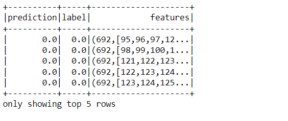
Inference: In the above output we have filtered the main DataFrame to extract the important columns only i.e. prediction, label, and features.

evaluator = MulticlassClassificationEvaluator(labelCol="label", predictionCol="prediction", metricName="accuracy")

Inference: Here we are in the stage of model evaluation and for that, we are using the Multi-class classification Evaluator there is one key difference between Binary and Multi-class evaluators, binary on one side can only return the AUC curve while the other one can return the accuracy, precision and recall metrics as well.

accuracy = evaluator.evaluate(predictions)
print("Test Error = %g" % (1.0 - accuracy))

Output:

Test Error = 0

Inference: Well!! to get the 0 test error seems to be a bit unacceptable especially in the real setup, having said that keep one thing in mind this dataset is highly separable and cleaned so one might expect such tremendous results.

Gradient Boosted Trees

Gradient boosting Trees (GBTs) is another tree method that can be used for both classification and regression problems GBTs are built based on ensemble methods using several decision trees. Though one doesn’t have to worry about the mathematics behind this algorithm as Spark handles it in a better way.

from pyspark.ml.classification import GBTClassifier

data_gbt = spark.read.format("libsvm").load("sample_libsvm_data.txt")

(trainingSet, testSet) = data_gbt.randomSplit([0.7, 0.3])

gbt_mdl = GBTClassifier(labelCol="label", featuresCol="features", maxIter=10)

model = gbt_mdl.fit(trainingSet)

predictions = model.transform(testSet)

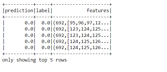
predictions.select("prediction", "label", "features").show(5)

Output:

 

Code breakdown: This is just for the walkthrough purpose otherwise if you have learned the random forest part then this one will be easy to pick up in terms of implementation.

1. Firstly importing the GBT model and reading the dataset by the same method.
2. Splitting the dataset into training and testing sets using the random split method.
3. Training of the GBT model using object creation and fit method.
4. Making predictions using the transform method on testing data.

evaluator = MulticlassClassificationEvaluator(labelCol="label", predictionCol="prediction", metricName="accuracy")
accuracy = evaluator.evaluate(predictions)
print("Test Error = %g" % (1.0 - accuracy))

Output:

Test Error = 0.0625

Inference: As we did in the case of random forest similarly following the same approach for GBT where we got the test result as around 0.088 which seems a bit realistic.

Note: The same pipeline can be applied in the case of the decision tree as well.

Conclusion to MLIB

In this article, we have discussed all the important tree methods that can be implemented using PySpark’s MLIB and went through the hands-on practice by using the official documented dataset provided by Spark. Now, let’s discuss everything we did in a nutshell.

1. First, we did an environment setup thing and read the dataset and then look at the dataset which was preprocessed and ready to use for model development.
2. Then the stage of splitting the dataset comes into existence followed by the random forest model development, prediction, and in the end evaluation.
3. Similarly, we perform the same process in the case of the GBT model (practically) and conclude that using any tree method need to follow the same process.

Here’s the repo link to this article. I hope you liked my article on Introduction to tree methods in MLIB. If you have any opinions or questions, then comment below.

Connect with me on LinkedIn for further discussion on MLIB or otherwise.

The media shown in this article is not owned by Analytics Vidhya and is used at the Author’s discretion.