This article was published as a part of the Data Science Blogathon.
Introduction
In this article, we will be working withPySpark‘s MLIB library it is commonly known as the Machine learning library of PySpark where we can use any ML algorithm that was previously available in SkLearn (sci-kit-learn). We can perform all the operations which were required in the complete ML pipeline.
Starting the Spark Session
The very first step before playing with PySpark is to set up and start the Spark session and for that, we will be first importing the SparkSession function from the pyspark.sql package.
from pyspark.sql import SparkSession

df_ml = SparkSession.builder.appName('Machine learning example').getOrCreate()
df_ml
Output:
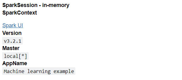
Inference: After importing the SparkSession function, we used the builder function to build our session and gave the name to the session using the appName function, which is under the builder function only at the last, we simply created the session using the getOrCreate() function.
Reading the Dataset

Before heading towards reading the data, let’s understand what our dataset is!
So this dataset is a banknote authentication dataset from Kaggle, and it holds the statistical details of both real notes and fake notes. IF you wanna know more about this dataset, follow this link.
Feature columns:
- Variance
- Skewness
- Kurtosis
- Entropy
Target column:
- Target
Now, after creating and setting up the SparkSession it’s time to read the dataset on which we will be applying machine learning operations and, before that, the data preprocessing techniques using PySpark.
training_dataset  = df_ml.read.csv('/content/bank_notes.csv', header=True, inferSchema=True)
training_dataset
Output:
DataFrame[variance: double, skewness: double, curtosis: double, entropy: double, Target: int]
Inference: Here, with the help of the read.csv() function, we have read the CSV formatted dataset and provided the header as True so that we can get the column name as header and infer schema as True so that we can get the real data type each column.
Let’s see our dataset now
training_dataset.show()
Output:
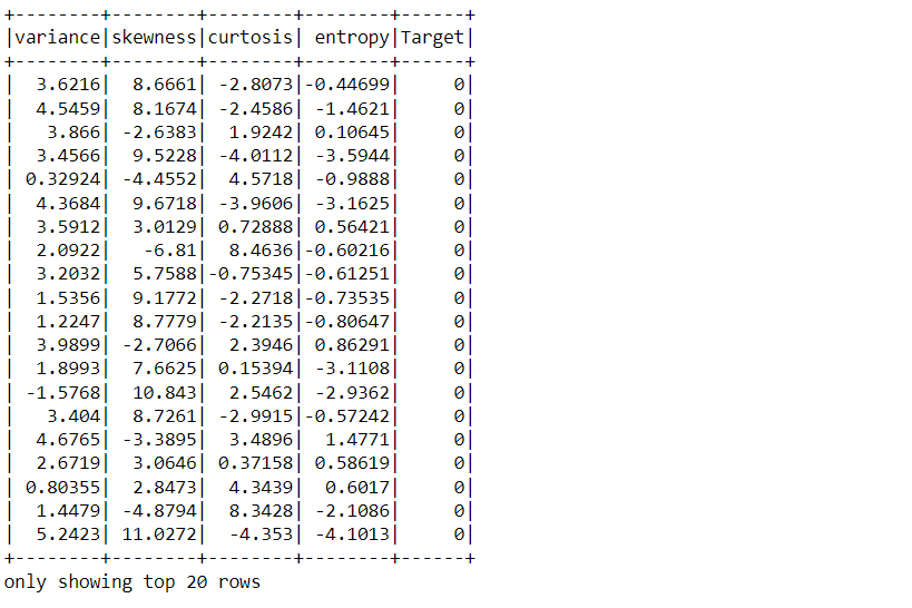
Inference: Here, we can see the top 20 rows of the dataset with the help of the show() function
Now we will look at the Schema of our banknote detection dataset i.e. we will see what data type each column hold and do it has null values or not? So let’s answer this question with the printSchema() function.
training_dataset.printSchema()
Output:
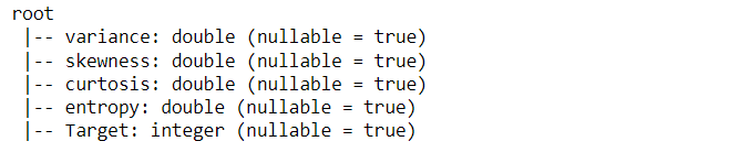
Inference: After calling the printSchema method, we can see that it returned the type of the data of each column where:
- Variance, Skewness, Kurtosis, and Entropy column holds the double type value, which is our dependent columns, i.e. features and
- The target column has the integer type value, which is our independent column i.e. Target column.
Though by far, we saw the complete schema of our dataset, this is not something which we wanna see all the time instead, to see just how many columns are there, so let’s figure that out!
training_dataset.columns
Output:
['variance', 'skewness', 'curtosis', 'entropy', 'Target']
Inference: By using the columns object, we can see how many columns are there in the data, and it will be returned in the list format.
Vector Assembler
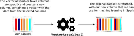
Vector assembler is the package that helps us to bring all the dependent columns, i.e. features, in one column; in short, it stacked the feature columns together in the form of vector type, so now, instead of dealing with multiple columns, we only need to care about that one column because it holds all the data which we need to train our model.
# ["variance", "skewness","curtosis", "entropy"] -------> new feature -------> independent feature
from pyspark.ml.feature import VectorAssembler

featassembler = VectorAssembler(inputCols=["variance", "skewness","curtosis", "entropy"], outputCol = "Independent Features" )
featassembler
Output:
VectorAssembler_835df549891f
Code breakdown:
- Firstly we have imported the VectorAssembler from the pyspark.ml.feature library.
- Then we used the same VectorAssembler to stack our dependent features together with the help of the following parameters.
- input-Cols: This parameter will hold all the features in the form of a list on which we are aiming to perform ML operations.
- output-Col: Here, we will give the name to the column to which we are grouping all the features.
Transforming the Dataset
In this section we will transform our dataset i.e. we will add our Independent feature columns to the original dataset as we all know that the ML algorithm should have clean and sorted data so data transforming is a must-do step.
result = featassembler.transform(training_dataset)
result.show()
Output:
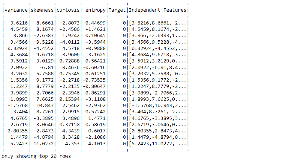
Inference: So, by using the transform() over the assembler object, we have successfully added the independent feature(S) column at the last column(from left)
Technically thinking so now our dataset should hold one more column i.e. The independent feature column; let’s check that using our columns object on the variable that holds the resultant dataset.
result.columns
Output:
['variance',
 'skewness',
 'curtosis',
 'entropy',
 'Target',
 'Independent Features']
Yes, it does! we have our last column in the dataset but do we need the other columns like Kurtosis, variance, skewness, and entropy?
No right! because these columns we already have in the last column that we created using the Vector Assembler method. So, in the end, we should only have 2 columns from the dataset, and they are:
- Independent features: That holds all the features which we need to apply the machine learning algorithm
- Target: That holds the result and from which we will be checking our prediction.
Here we are doing it, we are simply making a final dataset that will consist of only 2 columns.
final_data = result.select("Independent features", "Target")
final_data.show()
Output:
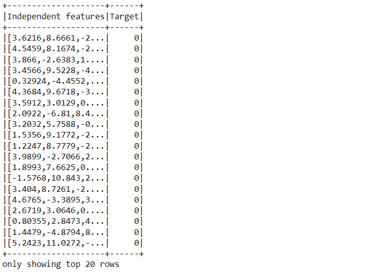
Inference: Nowhere with the help of select() we filtered out the grouped feature column as well as the resultant column, and now are dataset only have 2 columns, and these are the only one that we care for now.
Train Test Split
Now, as we know, the Train Test split is one of the known steps in the machine learning pipeline where we divide our training dataset and testing dataset to remove the problem of overfitting of the model as if we will train the model on the whole dataset then it will undoubtedly lead to the problem of overfitting of the model hence we should always divide the data into training and testing sets.
In PySpark, we will be using the random split() function to divide the data into training and testing sets.
train_data, test_data = final_data.randomSplit([0.75, 0.25])
Inference: Now as we can see that we are breaking up the data into 75% of training and 25% of testing data using the random split() function and it is getting stored in the train_data and test_data variables simultaneously.
Model Building
Now, as if we have split our dataset and already have our training set, so it’s time to build our model based on the training dataset and then test the same model corresponding to the testing data. As we know that it is a regression problem so we will be using the Linear Regression algorithm.
from pyspark.ml.regression import LinearRegression

model = LinearRegression(featuresCol = 'Independent features', labelCol='Target')
model = model.fit(train_data)
Code breakdown:
- Firstly we have imported the LinearRegression algorithm from the pyspark.ml.regression package.
- Then we will define our independent features and target column after specifying the feature-Col and label-Col simultaneously.
- After defining the feature columns and target, we will fit our training data with the model that we have created.
Coefficients and Intercepts
The one who knows about the mathematical intuition of linear regression can easily pick up what this coefficient and intercepts demonstrate. For the ones who are not aware of the same for them, we will discuss it in nutshell.
Equation of linear regression: y = c + b*x Where,
- “y” is the dependent variable i.e. target variable.
- “x” is the independent variable i.e. features.
- “b” is the slope of the line and is also known as the regression coefficient
- “c” is the intercept which is also known as the constant.
Coefficients
model.coefficients
Output:
DenseVector([-0.142, -0.0786, -0.1014, 0.0])
Inference: In the output, we can see that it has given us the array of a list of coefficients in the form of Dense Vector i.e. all the regression coefficients in the Vector format.
Intercepts
model.intercept
Output:
0.7994252652531315
Inference: In the output, we can see the intercept that our model has and it represents the mean of the target variable when all the feature variables collectively have zero value.
Predicting the Results
So here we have come to the section where we will see how our model performed after all the training it went through, and we call it the Prediction section.
prediction_result = model.evaluate(test_data)
prediction_result
Output:
Inference: Here for predicting the results we are using the testing data and along with that involving the evaluate() method to predict the results on that unseen data then in the output we can see that it returned the object of ml. regression.LinearRegressionSummary.
prediction_result.predictions.show()
Output:
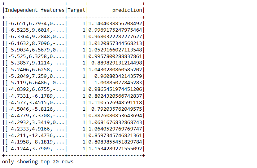
Inference: Now, with the help of the show method, we can easily compare how close are the predicted value than the actual value and it returns the DataFrame where we can see the predicted as well as actual values side by side based on the DataFrame we build previously.
Conclusion
In this section, we will summarize in a nutshell whatever we have covered so far, firstly we started our spark session and imported the banknote authentication dataset. Later, we also learned about Vector Assembler and implemented the same the last, we followed various steps in the ML pipeline to make predictions.
- First, we have completed our mandatory steps of starting the spark session and reading the banknote dataset.
- Then we used Vector Assembler to stack all our feature columns.
- Then we have transformed the dataset so that it could lead to clear and understandable results.
- Later we used the random split() method to split our dataset into training and testing data
- Then we build our linear regression model using the fit method and found the coefficients and intercepts of the model
- Finally, we draw the prediction that our model has predicted based on the testing data.
Here’s the repo link to this article. I hope you liked my article on Introduction to PySpark MLIB. If you have any opinions or questions, then comment below.
Connect with me on LinkedIn for further discussion.
The media shown in this article is not owned by Analytics Vidhya and is used at the Author’s discretion.


