Sentiment Analysis with Focus on the Naive Bayes Classifier

This article was published as a part of the Data Science Blogathon.

Introduction to Naive Bayes Classifier

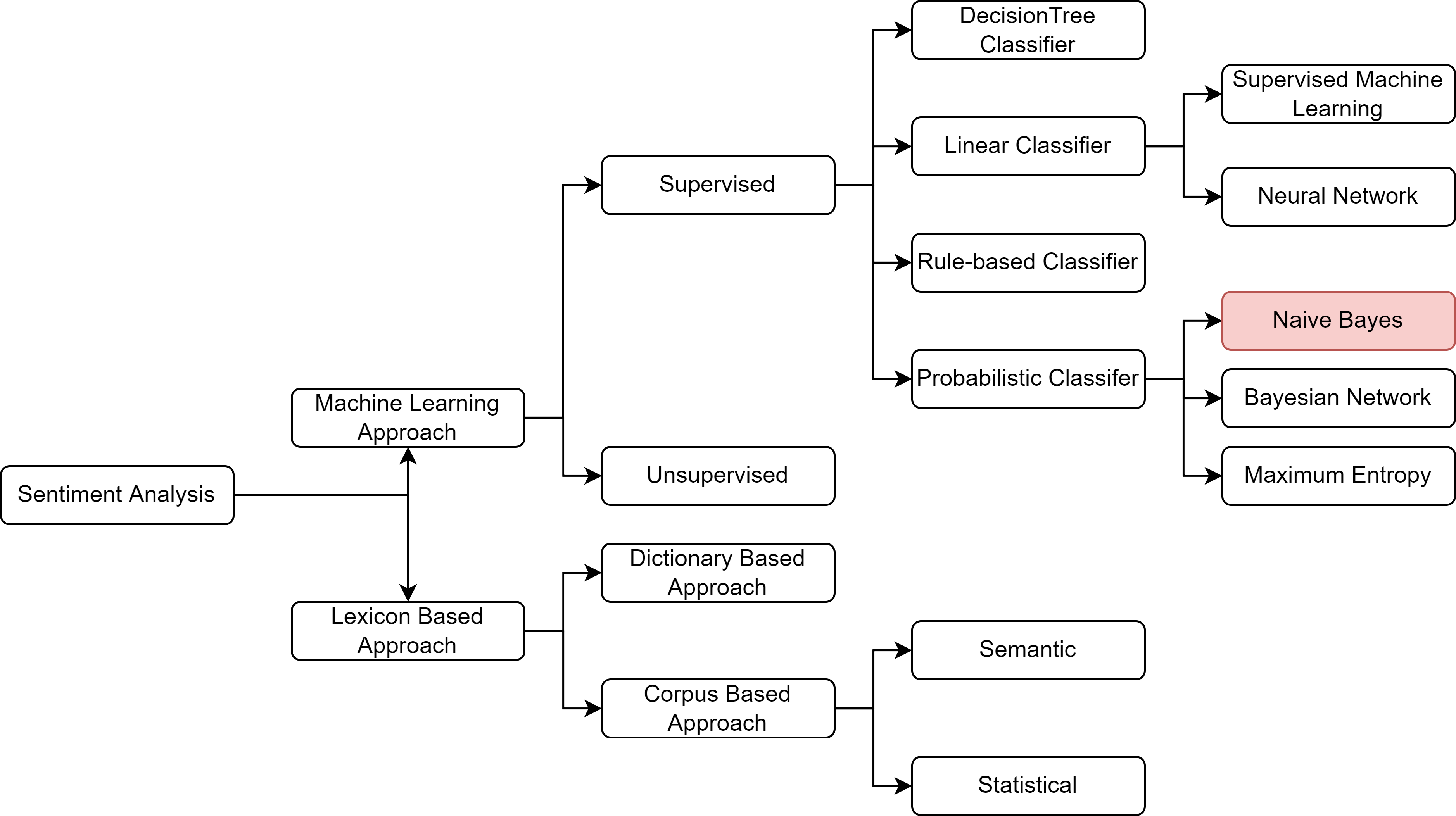
Sentiment Analysis, alternatively known as “Opinion Mining,” has been buzzing recently. And researchers worldwide are constantly focussing on developing newer techniques and architectures that would allow easy detection of the underlying tone or sentiment of a particular text. With the exponential growth of social websites, blogging sites, and electronic media, the amount of sentimental content in the form of movies or product reviews, user messages or testimonials, messages in discussion forums, etc., has also increased. Timely discovery of these sentimental or opinionated messages can potentially reap huge advantages – the most crucial being monetization. A better understanding of the sentiments of the masses towards products or services allows for better analysis of market trends, contextual advertisements, and ad recommender systems. While in the contemporary scenario, many advanced machine learning techniques and pipelines exist for sentiment analysis, it is always good to be aware of the basics. So the goal of this article would be to provide a mathematical yet detailed idea of the intricacies of one of the oldest workhouses of machine learning: the Naive Bayes’ (NB) Classifier.

The Bayes’ Theorem

The NB Classifier stems from the fundamental concept of Bayesian statistics – the conditional probability and Bayes’ Theorem. The article expects the readers to be foundationally strong with the basic definitions of probability. So it is advised to recall those definitions and formulas before proceeding further.

The definition of conditional probability or the probability of the occurrence of event A given event B, denoted by P(A|B), is given by the joint probability P(A ∩ B) divided by the marginal probability P(B

Where Ω denotes the sample space.

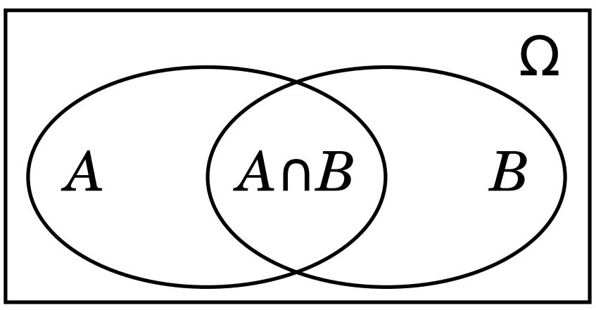
Figure 2: Showing the intuition behind conditional probability

To think intuitively, as in figure 2, what would be the probability of being in ellipse A, given that you are already in ellipse B? Your answer would be that to
be also in A, we must be in the intersection (A∩B). Hence, the probability is equivalent to the number
of elements in the intersection (A∩B), divided by the number of elements in B, i.e., (B). Thus we have the formula for conditional probability as already stated.

Now assuming A and B are non-empty sets, for both A and B w can write,

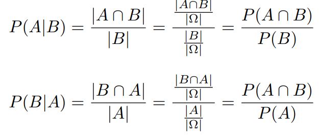
We can rearrange the above two equations to write.

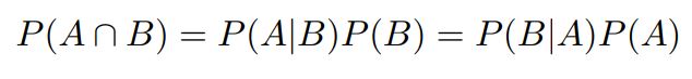
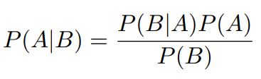
Rearranging the above equation, we get the final form of the Bayes’ theorem as

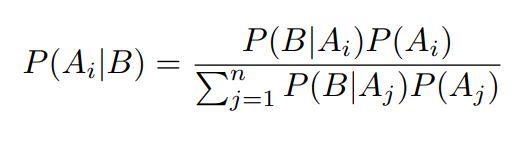
If the sample space can be divided into n number of mutually exclusive events, and if B
is an event with P(B) > 0, which is a subset of the union of all A_i, then for each A_i, the generalized Bayes’
formula is

The Naive Bayes Classifier

The Naive Bayes’ (NB) Classifier is a well-known Bayesian network classifier paradigm of a supervised classification model. The NB is a probabilistic classifier based on the Bayes’ Theorem considering the naive independence assumption. It was earlier introduced under a different name in the NLP community. It remained a popular baseline model for text categorizing, the problem of judging documents as belonging to one category or the other. The advantage of NB is that it requires less training data to estimate the parameters necessary for classification. With its fundamental driving formula being the Bayes’ theorem and the conditional probability model, the NB model, despite its simplicity and solid and robust assumptions, proves quite effective in most use cases, especially in the field of NLP, as we will see in the next section. Before that, it would be worthwhile to look into the assumptions that NB considers for classifying and how they affect the output from the perspective of NLP.

Assumptions of Naive Bayes Classifier

The NB classier mainly consider two assumptions that help reduce the model complexity.

1. It makes the independence assumption, whereby it assumes that the words in a corpus/ text are independent of each other, and there would exist no correlation between any two/group of words.

For example, consider the sentence “The Sahara desert is mostly sunny and hot.” Then, in that case, the word sunny and hot tend to depend on each other and are correlated to a certain extent with the word “desert.” Naive Bayes assumes independence throughout. This naive assumption is not always accurate and is one of the causes of low performance in some cases of the NB model.

2. It is heavily dependent on the relative frequencies of the words in the corpus taken into consideration. This sometimes leads to model inaccuracies, as existing datasets are usually noisy in the real world.

Now that we are thorough with the basic concept of NB and the assumptions, we are ready to see an application of the NB in sentiment analysis.

Naive Bayes Classifier in Sentiment Analysis

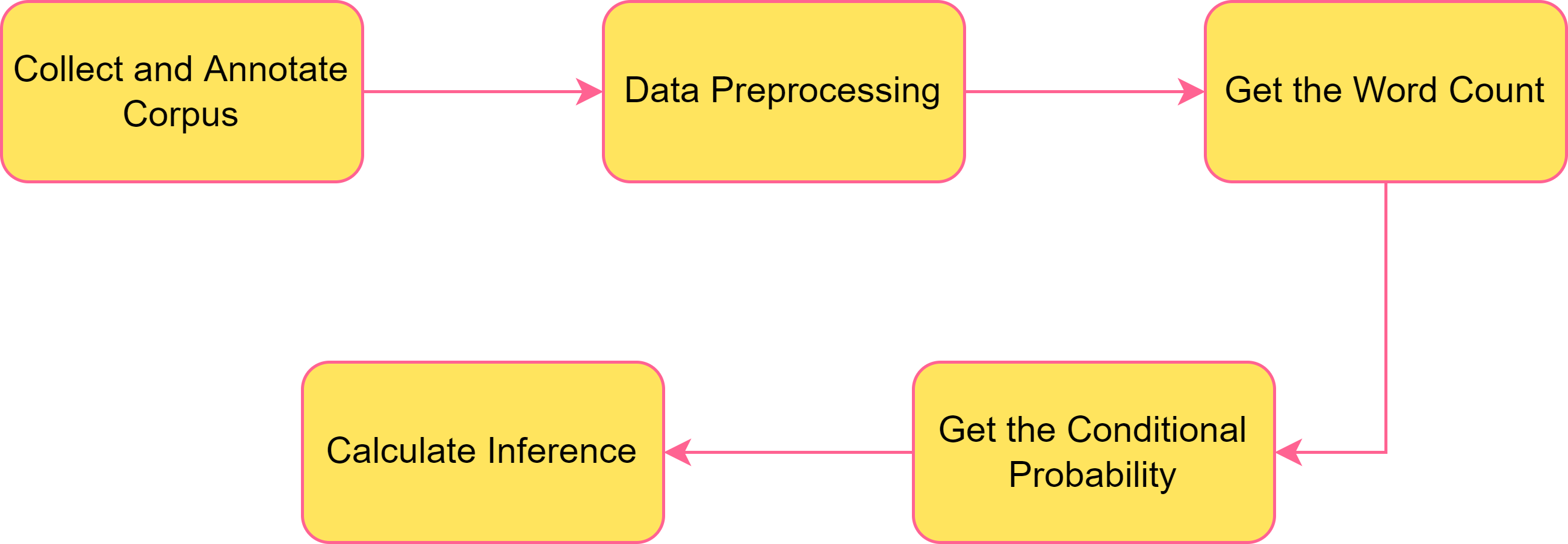
In this section of the article, we would be looking into how NB Classifier can be leveraged to carry out sentiment analysis. Figure 3 shows steps to build the desired model. Each of the mentioned steps will be explained in detail in the paragraphs that follow.

Step 1 Collect and Annotate Corpus

For the purpose of the dataset, let us consider a corpus of tweets where two are labeled positive tweets and two are labeled negative tweets. Obviously, the numbers considered are just to ensure an enhanced understanding of the concepts, real-world scenarios would include much more diverse situations. So in the corpus, as shown in Figure 4, the sentences “I am happy because I am playing chess” and “I am happy, not sad” are labeled as positive sentiments, and the sentences “I am sad, I am not playing chess” and “I am sad, not happy” are marked as negative sentiments.

Figure 4: Schematic representation of the corpus taken into consideration for this example walkthrough

Step 2 Preprocessing

This step is one of the most critical processes that need to be carried out prior to getting started with the model. The methods used in this step may vary from time and use but in general, in this step, you remove the punctuation marks and stop words, remove the handles and URLs in the text (if any), lowercase all the letters, and perform stemming on the entire text. The overall effect of the above methods is that they help reduce the vocabulary greatly and output a vector of words, which is then used in the further steps.

Step 3 Get the Word Count

In this step, first, we get a  total count of all the words in the positive and negative corpus and prepare a table as shown in Figure 5.

Step 4 Get the Conditional Probability

This is the step, where ultimately you can use the formulas that we had earlier derived at the starting of the article. This step makes use of the Bayes’ Theorem to calculate the probability of occurrence of the word.

With the word count table, we try to get the probability table, as shown in Figure 6. We divide each word in a class by its corresponding sum of words in the class to get the probability of occurrence of that particular word. For example, the word count of “I” in positive tweets is 3 and the total number of words in the positive tweets is 13. So the corresponding value of “I” in the frequency table would be (3/13=) 0.24. In a similar fashion, the entries in the other cells are filled up to complete the table. To put it formally, we calculate the probability of a word given a class by the below formula.

An important concept to note here is that words like “I“, “am“, “playing“, and “chess” have the same probability, or in other words they are equiprobable – they do not add anything to the sentiment (as they get canceled out while calculating the likelihood value, something we would cover in the following steps). On the other hand, words like “happy“, “sad“, and “not” possess significant differences between the probabilities. These are also known as power words and they carry a lot of weight in determining sentiment.

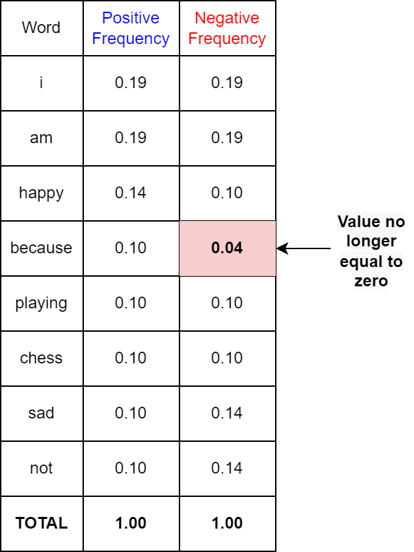
However, one flaw with the above method of assigning the conditional probabilities is that if a word does not appear in the training, then its probability of occurrence is automatically equal to zero. In order to tackle this problem, a new concept of Laplacian Smoothing is introduced, whereby the formula of Bayes’ theorem is tweaked slightly to avoid getting a zero probability. The modified formula taking into consideration the Laplacian Smoothing thus becomes

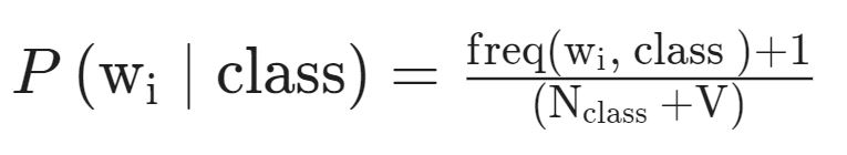
Where V denotes the number of unique words in the vocabulary. For the case considered, it is equal to 8.

The new probability table after considering the Laplacian smoothing thus becomes as shown in Figure 7. Note that the word “because” which had zero probability earlier in the negative class now has a non-zero probability.

Step 5 Calculate the Inference

Once the probabilities of each word are calculated, the last step that remains is to calculate a score that will allow us to decide whether a tweet is a positive or negative sentiment. An inference score greater than zero would denote a positive sentiment and a score less than zero would denote negative sentiment. A score equal to zero would denote neutral sentiment.

So, to get an inference about the result, we calculate the following :

where the first term is referred to as log prior and the second term as log-likelihood.

One thing to notice is that for a balanced dataset, where the amount of positive and negative data are equal, the log prior would be zero. Then calculating the likelihood only would suffice the inference.

Conclusion

We now have successfully walked through the steps required to train a Naive Bayes’ Classifier model and are in a position to get started on implementing this.

To recapitulate, the key takeaways from the article are:

1. First we started with a brief discussion on Sentiment Analysis and the various algorithms that can be used to achieve the same.

2. Then we briefly discussed the Bayes’ Theorem, which is the principal equation governing the Naive Bayes’ Classifier.

3. The following section discussed extensively the Naive Bayes’ (NB) Classifier and the assumptions leading to the model.

4. The last section dealt with implementing an NB classifier and we learned the various steps to develop the model along with the practical implementation of the various calculations involved in building the NB Classifier.

I hope this article gave you a clear understanding of the NB classifier. I would recommend you to further go ahead and do a practical implementation of the model with a real-world dataset to gather a more rigid understanding of the same. Go quick and try your hands at recommender systems with real-world datasets!

The media shown in this article is not owned by Analytics Vidhya and is used at the Author’s discretion.

Neil D

Neil is a research professional currently working on the development of AI agents. He has successfully contributed to various AI projects across different domains, with his works published in several high-impact, peer-reviewed journals. His research focuses on advancing the boundaries of artificial intelligence, and he is deeply committed to sharing knowledge through writing. Through his blogs, Neil strives to make complex AI concepts more accessible to professionals and enthusiasts alike.