This article was published as a part of the Data Science Blogathon.
Introduction
While reading the heading of this article, one has surely got to know that this will gonna be the advanced topic with regards to SVM – The supervised machine learning algorithm capable of implementing both classification and regression problem statements. But no worries, I’ve got your back s before jumping straight to SVM’s Kernels, I’m gonna make sure that you all have an understanding of the basic terminologies related to SVM in general to develop a generalized model but not an overfit model.
What is SVM?
As mentioned earlier, SVM is a supervised ML algorithm that stimulates, it will always have the labeled dataset for regression or classification. The one who knows about the mathematical intuition of logistic regression can surely relate to the concept of Hyperplane as in SVM also we use hyperplanes to classify the opponent and considered class. But SVM is way ahead with logistic regression because,
SVM has the concept of Margins which are supported by the vectors. Vectors are nothing but the closest data point from their opponent class. The main aim of margins is to provide some cushion to the model to develop a generalized model that can correctly predict the unseen data by removing the overfitted model’s drawback.
Why do we Need SVM Kernels?
So we have discussed a lot about the basics of SVM; let’s discuss the last thing here: When we have the absolute linearly separable dataset with us, then the SVM classifier can simply draw the hyperplane to classify the components, but in the real world, it’s tough to get the completely separable dataset so in that situation where we have a radial surrounded data points, or that cannot be easily separated with just a single hyperplane then comes the role of SVM kernels that helps in converting the lower dimension to higher dimensions also introducing some extra components (features) making it a technique worth separating the radial dataset.
There are many options from which we can select the SVM kernel based on the problem statement, though mainly three have the more weightage in most of the analysis:
- Polynomial kernel
- Sigmoid kernel
- RBF kernel
In this article, we will discuss the polynomial kernel for implementation and intuition.
import numpy as np
import matplotlib.pyplot as plt
import pandas as pd
from sklearn.svm import SVC
from sklearn.metrics import accuracy_score
In the above lines of code, we started our practical implementation by importing all the essential libraries:
- Numpy: For performing all the mathematical calculations (here, transpose of a matrix).
- Matplotlib: To show the data points we are giving as a dataset in the form of plots.
- Pandas: To convert those NumPy-created data points into structured DataFrames.
- SVC: It is the Support Vector classifier used only for classification.
- Accuracy Score: This library is needed to check how well our model performed.
x = np.linspace(-5.0, 5.0, 100)
y = np.sqrt(10**2 - x**2)
y=np.hstack([y,-y])
x=np.hstack([x,-x])
x1 = np.linspace(-5.0, 5.0, 100)
y1 = np.sqrt(5**2 - x1**2)
y1=np.hstack([y1,-y1])
x1=np.hstack([x1,-x1])
Inference: Creating the (x,y) and (x1,y1) coordinates to develop the plot which has data points in a radial manner or data points are clustered around a center position so that it makes us use SVM kernels as such type of distribution is not easily separated by a linear hyperplane.
plt.scatter(y,x)
plt.scatter(y1,x1)
Output:
Hit Run to see the output
Inference: In the above plot, one can notice the impact of using the sqrt( radius – x^2), which has spread the blue data points away from the elliptical-shaped orange data points (radial).
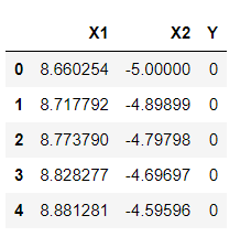
df1 =pd.DataFrame(np.vstack([y,x]).T,columns=['X1','X2'])
df1['Y']=0
df2 =pd.DataFrame(np.vstack([y1,x1]).T,columns=['X1','X2'])
df2['Y']=1
df = df1.append(df2)
df.head(5)
Output:
Inference: It’s time to rearrange the created data points in the form of DataFrames so that we can easily manipulate and get carry forward with our further analysis. Here we are using Transpose (T) as per the equation of the hyperplane. And with the help of NumPy, we are easily calculating the dot product of two matrixes (x,y, and x1,y1) which is part of the hyperplane calculations.
Independent and Dependent Features
Now it’s time to separate our dependent and independent features, and we are going to achieve this feat using pandas’ ILOC function, where we are taking everything from starting to the second last column and storing it in X (independent) while keeping the last column in y (dependent).
BLOG
Output:
Split the Dataset into Train and Test
We have separated the dependent and independent data as just in our previous code. Now, it’s time to split the data into training and testing. Training data will be used in the model building phase, while testing data will be considered to analyze how well our model performed.
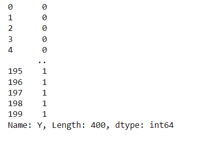
from sklearn.model_selection import train_test_split
X_train,X_test,y_train,y_test=train_test_split(X,y,test_size=0.25,random_state=0)
y_train
Output:
Inference: Keeping the testing size at 25% and the random state at 0 (so that each time the model is trained, it should get the same sample data), we have successfully split our dataset according to the machine learning pipeline.
classifier=SVC(kernel="linear")
classifier.fit(X_train,y_train)
Output:
SVC(kernel='linear')
y_pred = classifier.predict(X_test)
accuracy_score(y_test, y_pred)
Output:
0.45
Inference: Note that, for comparison purposes, we have first used the linear kernel, knowing that for this type of dataset, it is way too hard to classify the components. Just by using a linear hyperplane, we can also see the model’s accuracy as 45%, which will never be accepted in a real-world setup.
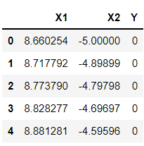
df.head()
Output:
Inference: One more thing to keep an eye on is that in the linear kernel, we just have 2 features to work with, i.e., lower dimension. Now comes the interesting part, where we will see how the polynomial kernel will help in converting the lower dimension feature set to the higher dimension.
Polynomial Kernel
Polynomial kernels widely opt kernels while we need to have the conversion from lower to higher dimension data especially when we are working with the dataset that is radial, i.e., for such data, it is very hard to classify the results using linear hyperplanes in that case, polynomials, RBF and sigmoid kernels come to rescue.
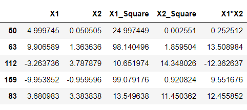
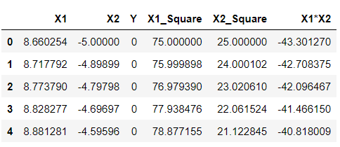
df['X1_Square']= df['X1']**2
df['X2_Square']= df['X2']**2
df['X1*X2'] = (df['X1'] *df['X2'])
df.head()
Output:
import numpy as np
import matplotlib.pyplot as plt
import pandas as pd
from sklearn.svm import SVC
from sklearn.metrics import accuracy_score

x = np.linspace(-5.0, 5.0, 100)
y = np.sqrt(10**2 - x**2)
y=np.hstack([y,-y])
x=np.hstack([x,-x])


x1 = np.linspace(-5.0, 5.0, 100)
y1 = np.sqrt(5**2 - x1**2)
y1=np.hstack([y1,-y1])
x1=np.hstack([x1,-x1])

plt.scatter(y,x)
plt.scatter(y1,x1)
plt.show()
Inference: Just by looking at the above output, one will identify my meaning of higher dimensions as now we can see that we have 5 components, unlike previously when we got only 2 and this we have achieved by simply applying mathematics behind SVM’s polynomial kernels, i.e., square of X1 and X2 gave us 2 extra features, similarly with X1.X2. These are all we have achieved by the above equation- (x.T*y +c)^d.
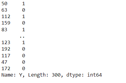
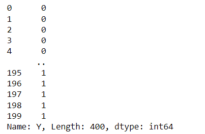
X = df[['X1','X2','X1_Square','X2_Square','X1*X2']]
y = df['Y']
y
Output:
X_train, X_test, y_train, y_test = train_test_split(X, y,
test_size = 0.25,
                                                    random_state = 0)
X_train.head()
Output:
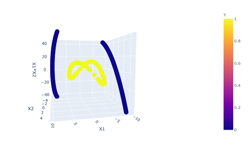
import plotly.express as px

fig = px.scatter_3d(df, x='X1', y='X2', z='X1*X2',
              color='Y')
fig.show()
Output:
Inference: Here, we opted to go with PLOTLY library as we are working with more than 2-D data so it will be more interactive to see the changes. In the above plot, one can notice that we have a slight improvement by choosing only 2 more features from the new ones, but still, this data is not separable.
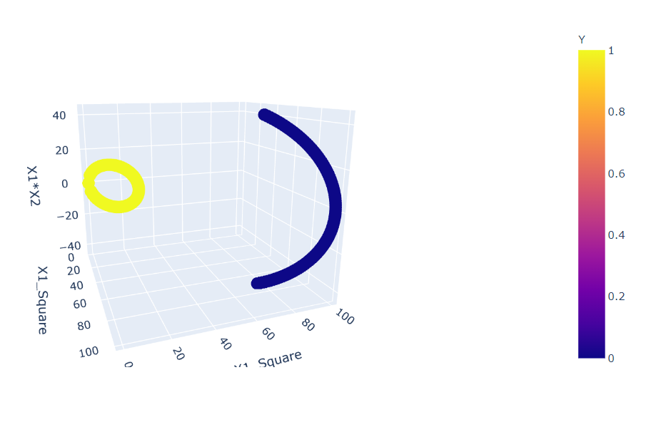
fig = px.scatter_3d(df, x='X1_Square', y='X1_Square', z='X1*X2',
              color='Y')
fig.show()
Output:
Inference: Before plotting this graph, we changed our components to X1_square and X2_square from X1 and X2, and as a result, we can see that now we have the distribution of points that can be easily separable by just using a linear plane.
classifier = SVC(kernel="rbf")
classifier.fit(X_train, y_train)
y_pred = classifier.predict(X_test)
accuracy_score(y_test, y_pred)
Output:
Inference: The above code is just to let you know that python’s sklearn library can help you do all the steps in just a chunk of code, but it is equally important to know what is happening in the background which is also the sole purpose of this article.
Conclusion
Here we are in the end game now. In this article, we got to learn what SVM kernels are, when we will use them, and how these kernels can help us get out of the hectic situation like dealing with the radial datasets. Here I’m trying to list everything we got through in this article.
- The first step we answered ourselves is the what, when, and how questions about the SVM kernels so that before practically implementing it, we should understand its basics.
- Then we move to the practical side of the same, where we used simple linear kernels for experiment purposes to see how badly it could perform (while looking at the accuracy) and as expected, it only had 45% accuracy.
- At last, we finally build the model again using polynomial SVM kernel and plotted that too. Both graphs and accuracy level made us believe that it is always good to go with SVM kernels for such complex data.
Here’s the repo link to this article. I hope you liked my article on the Data visualization guide for multi-dimensional data. If you have any opinions or questions, then comment below.
Connect with me on LinkedIn for further discussion.
The media shown in this article is not owned by Analytics Vidhya and is used at the Author’s discretion.


