Analyzing and Comparing Deep Learning Models
This article was published as a part of the Data Science Blogathon.
Deep Learning Overview
Deep Learning is a subset of Machine Learning. Deep Learning is established on Artificial Neural Networks to mimic the human brain. In deep learning, we add several hidden layers to gather the most minute details to learn the data for predictive modeling.
Deep Learning is ANN. Previously, lack of processing power was not everyone’s cup of tea. With today’s exponential increase in processing power, implementing Deep Learning is a buzz.
Deep Belief Networks, Deep Neural Networks, and Recurrent Neural Networks are some of the Deep Learning Models. In this article, we will be comparing three models comprising CNN (Convolution Neural Network), DNN (Deep Neural Network), and LSTM (Long Short-Term Memory).

Table of contents
- Deep Learning Overview
- Dataset Affirmation
- Libraries Pre-requisites
- Data Exploration
- Loading Data
- Define Model 1 – DNN (Deep Neural Network)
- Define Model 2 – RNN (LSTM)
- Define Model 3 – CNN (Convolution Neural Network)
- Prediction Phase
- Comparing Model Accuracies
- What are the steps to creating and training deep learning models?
- Conclusion
- Frequently Asked Questions
Dataset Affirmation
Here we will use the MNIST dataset of handwritten digits ranging from 0 to 9. This dataset will be split into two parts, i.e., the training set and the testing set for prediction. Using the sklearn library, the MNIST dataset will be imported into the Jupyter notebook.
Source: https://en.wikipedia.org/wiki/MNIST_database
Implementation
The implementation is done in the Jupyter Notebook. The entire implementation is available on my Kaggle. The link is mentioned below:
Notebook Link: https://www.kaggle.com/code/shibumohapatra/cnn-dnn-lstm-comparison
Libraries Pre-requisites
To begin with, first, we will be importing libraries for the algorithm. Libraries and their use are mentioned below:
- Numpy: to work with arrays
- Pandas: data processing
- TensorFlow: model tracking for prediction
- Matplotlib: to plot graphs
- Keras: API for TensorFlow
- Tensorflow.keras.models: to build a machine learning model. We will import Sequential ( a stack of layers with only one input tensor and one output tensor).
- Sklearn.model: to split the data into a training set and a test set
- Tensorflow.keras.layers: importing different layers to implement deep learning. The description of the layers is mentioned below –
- Dense: creating feed-forward neural networks, meaning that every input and every output is dependent reciprocally.
- Flatten: serializing multi-dimensional tensor.
- Dropout: to prevent overfitting.
- conv2D: a 2D convolution layer to maintain the relation between pixels of image data.
- MaxPooling2D: reduce the spatial size.
from tensorflow.keras.models import Sequential
from tensorflow.keras.layers import Conv2D, MaxPooling2D, Dense, Flatten, Dropout, LSTM
from tensorflow.keras.utils import normalize
from sklearn.model_selection import train_test_split
Data Exploration
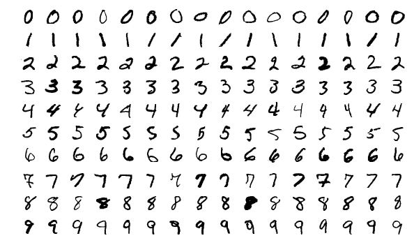
Here we will be loading the MNIST data and splitting it into 4 sets train_x, train_y, test_x, and test_y sets. After that, we will normalize the train_x and test_x sets and print their respective data shapes. Then we will display the dataset to ensure the exploration is right. I have implemented a for loop to plot 4 images of the dataset.
from keras.datasets import mnist
(train_x, train_y), (test_x, test_y) = mnist.load_data()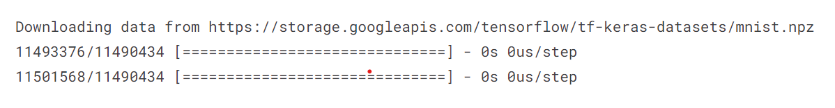
train_x = train_x.astype('float32')
test_x = test_x.astype('float32')
train_x /= 255
test_x /= 255
train_x = train_x.reshape(train_x.shape[0], 28, 28, 1)
test_x = test_x.reshape(test_x.shape)
# train set
print("The shape of train_x set is:",train_x.shape)
print("The shape of train_y set is:",train_y.shape)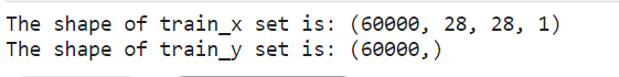
Train set the shape of the MNIST dataset
# test set
print("The shape of test_x set is:",test_x.shape)
print("The shape of test_y set is:",test_y.shape)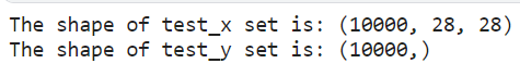
The test set the shape of the MNIST dataset
for i in range(1):
  plt.subplot(330 + 1 + i)
  plt.imshow(train_x[i].reshape(28,28), cmap=plt.get_cmap('gray'))
  plt.axis('off')
  plt.show()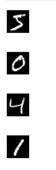
First four handwritten digits from the MNIST dataset
Loading Data
Once we implement data exploration further, we have to load the MNIST dataset and divide it into 4 parts x_train, y_train, x_test, and y_test. Then, normalize its training and testing set to maintain its integrity. And then return the normalized train and test sets.
Loading data for DNN and RNN (LSTM)
We will load the data for DNN and RNN (LSTM) by the def load_data_NN() function, load the dataset and perform normalization.
def load_data_NN():
  # load mnist dataset
  mnist = tf.keras.datasets.mnist  # 28 x 28 images of 0-9
  (x_train, y_train), (x_test, y_test) = mnist.load_data()
  # normalize data
  x_train = normalize(x_train, axis = 1)
  x_test = normalize(x_test, axis = 1)
  return x_train, y_train, x_test, y_test
Loading data for CNN
For CNN, we will define the def load_data_CNN() function, load split the dataset, and reshape the train and test sets.
In CNN, the need for reshaping is because it includes a convolution layer, max-pooling, flattening, and dense layers. Here train and test sets are reshaped into 28 x 28 x 1 (28 rows, 28 columns, 1 color channel).
def load_data_CNN():
  # load mnist dataset
  mnist1 = tf.keras.datasets.mnist  # 28 x 28 images of 0-9
  (x_train, y_train), (x_test, y_test) = mnist1.load_data()
  # reshape data
  x_train = x_train.reshape(x_train.shape[0], 28, 28, 1)
  x_test = x_test.reshape(x_test.shape[0], 28, 28, 1)
  # convert from integers to floats
  x_train = x_train.astype('float32')
  x_test = x_test.astype('float32')
  # normalize data
  x_train = normalize(x_train, axis = 1)
  x_test = normalize(x_test, axis = 1)
  return x_train, y_train, x_test, y_test
Define Model 1 – DNN (Deep Neural Network)
DNN is based on Artificial Neural Networks and has several hidden layers between the input and output layers. DNN is competent in modeling complex non-linear relationships. Here, the main purpose is to give input, implement progressive calculation on the input layer and display or present the output to solve problems. Deep Neural Networks (DNNs) are considered Feed Forward Networks in which data flows from the input layer to the output layer without going backward, and the links between the layers are one-way. This means this process goes forward without touching the node again.
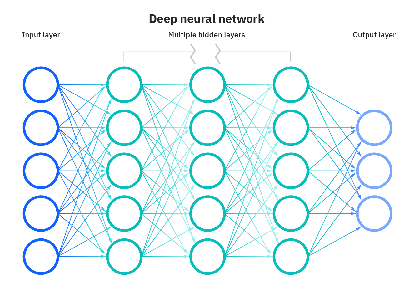
Source: https://www.ibm.com/cloud/learn/neural-networks
For the DNN – sequential, flattened, and 3 Dense layers are implemented. I have 128 nodes and a ReLU activation function for the first two dense layers. For the third dense layer, I have defined 10 nodes and a softmax activation function.
def DNN():
  model_dnn = Sequential()
  model_dnn.add(Flatten())  # input layer
  model_dnn.add(Dense(128, activation = 'relu'))
  model_dnn.add(Dense(128, activation = 'relu'))
  model_dnn.add(Dense(10, activation = 'softmax'))
  model_dnn.compile(optimizer= "adam",
                  loss= "sparse_categorical_crossentropy", metrics=["accuracy"])
  return model_dnn
Compiling the DNN model, I have used the Adam optimizer and sparse categorical cross-entropy (multi-class categorizing models in which the output label is assigned integer value) loss functions. The accuracy of the model will determine the metrics.
Define Model 2 – RNN (LSTM)
RNN is a short form of Recurrent Neural Network which is adapted to work for time series data or sequence data.
Here, we will be implementing LSTM, which is considered RNN. LSTMs (Long Short-Term Memory) is a special kind of RNN, capable of learning long-term dependencies, which makes RNN bright at remembering things that happened in the past to help make the next estimate sensible.
The use of LSTM resolves the problem of long-term dependencies of RNNs. The RNN could not store the word in long-term dependencies but based on recent information, the RNN could predict more accurately. But due to the increase in gap length, RNN fails to give optimal performance. The solution to this is done by LSTM, which retains the information for a long period, due to which data loss is decreased. The applications of LSTM are used for classifying time-series data and prediction.
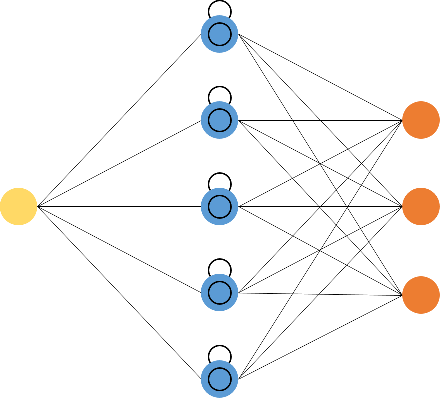
Source: https://i.stack.imgur.com/h8HEm.png
As for DNN (LSTM) – LSTM layer, sequential, Dropout Layer (will drop out 0.2 i.s. 20% of nodes to prevent overfitting), and Dense Layer. The above layers will have ReLU and softmax activation functions. Compiling the LSTM model, I have used the Adam optimizer and loss function (sparse categorical cross-entropy). The accuracy of the model will determine the metrics.
def RNN(input_shape):
  model_rnn = Sequential()
  model_rnn.add(LSTM(128, input_shape=input_shape, activation = 'relu', return_sequences=True))
  model_rnn.add(Dropout(0.2))
  model_rnn.add(LSTM(128, input_shape=input_shape, activation = 'relu'))
  model_rnn.add(Dropout(0.2))
  model_rnn.add(Dense(32, activation = 'relu'))
  model_rnn.add(Dropout(0.2))
  model_rnn.add(Dense(10, activation = 'softmax'))
  model_rnn.compile(optimizer= "adam",
                  loss= "sparse_categorical_crossentropy", metrics=["accuracy"])
  return model_rnn
Define Model 3 – CNN (Convolution Neural Network)
CNN is a category of Artificial Neural Networks. In Deep Learning, CNN is extensively used in object recognition and categorization. With the use of CNN, Deep Learning detects objects in an image. Convolutional Neural Networks (CNN, or ConvNet) is a class of deep neural networks most commonly applied to analyzing visual imagery. The applications of CNNs are video understanding, speech recognition, and NLP understanding. The CNN has an input layer, an output layer, one or many hidden layers, and tons of parameters, allowing CNN to learn intricate patterns and objects.
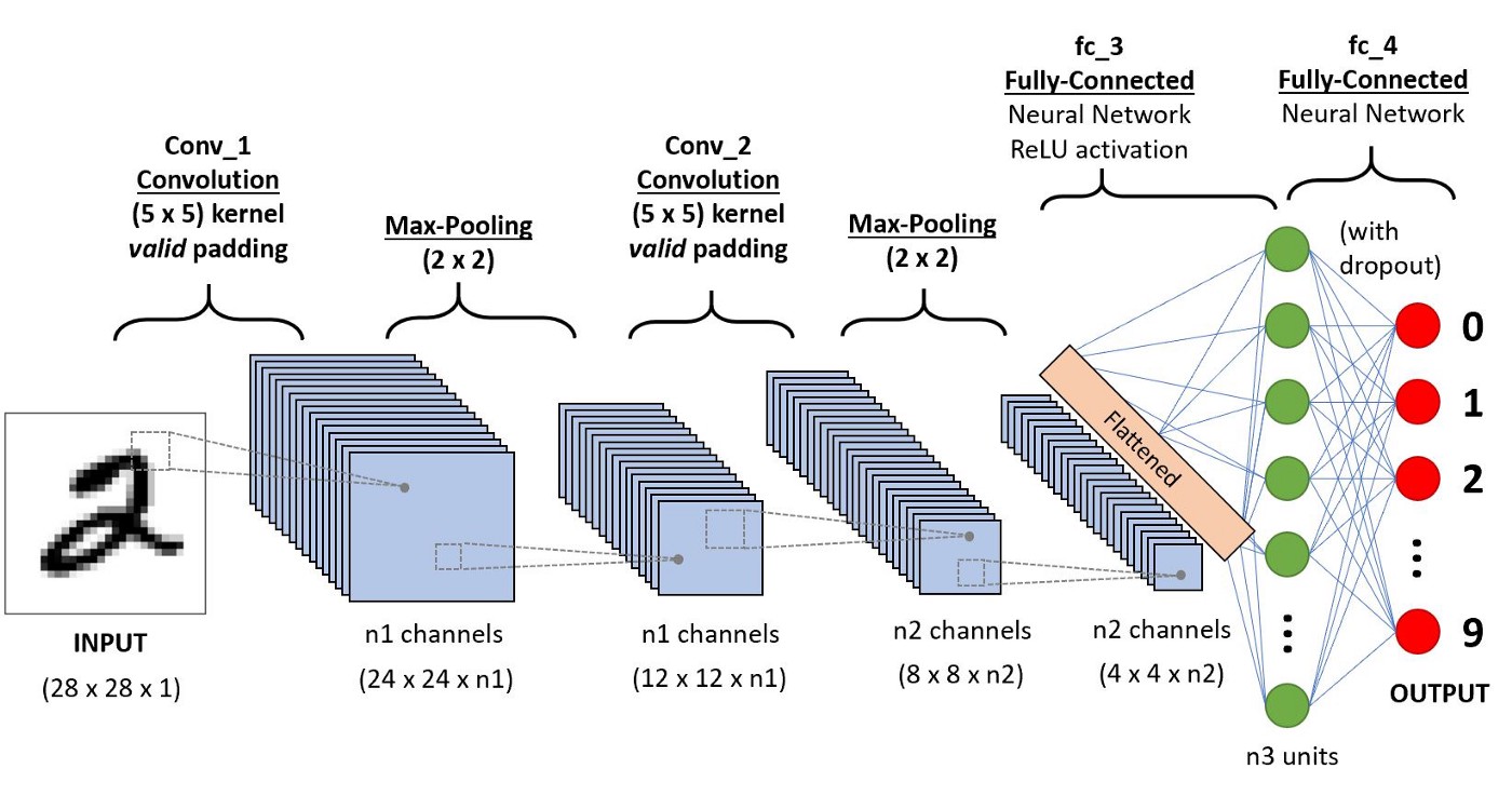
Source: https://miro.medium.com/max/1400/1*uAeANQIOQPqWZnnuH-VEyw.jpeg
For CNN, we will follow the Sequential, adding the Conv2D layer, MaxPooling2D Layer and Dense Layer. ReLU and softmax activation functions will be similar to the above models. Compiling the LSTM model, I have used the Adam optimizer and loss function (sparse categorical cross-entropy). The accuracy of the model will determine the metrics.
def CNN(input_shape):
  model_cnn = Sequential()
  model_cnn.add(Conv2D(32, (3,3),  input_shape = input_shape))
  model_cnn.add(MaxPooling2D(pool_size=(2,2)))
  model_cnn.add(Flatten())  # converts 3D feature maps to 3D feature vectors
  model_cnn.add(Dense(100, activation='relu'))
  model_cnn.add(Dense(10, activation='softmax'))
  model_cnn.compile(loss="sparse_categorical_crossentropy",
                 optimizer="adam", metrics=["accuracy"])
  return model_cnn
Prediction Phase
The below implementation helps us to predict and check the predicted output of a specific or distinct index of the image dataset.
Now, we can train and test the dataset with our built models.
def sample_prediction(index):
  plt.imshow(x_test[index].reshape(28, 28),cmap='Greys')
  pred = model.predict(x_test[index].reshape(1, 28, 28, 1))
  print(np.argmax(pred))
DNN Model Prediction
For DNN to predict first, we will load the load_data_NN() function, load, and fit the model with 5 epochs. After that model evaluation and test, accuracy is acquired, and finally, we will define a sample image to verify the model is predicting the image with maximum accuracy.
if __name__ == "__main__":
  # load data
  x_train, y_train, x_test, y_test = load_data_NN()
  # load the model
  model = DNN()
  print("nnModel Trainingn")
  model.fit(x_train, y_train, epochs = 5)
  print("nnModel Evaluationn")
  model.evaluate(x_test, y_test)
  score1 = model.evaluate(x_test, y_test, verbose=1)
  print('n''DNN Model Test accuracy:', score1[1])
  print("nnSample Prediction")
  sample_prediction(20)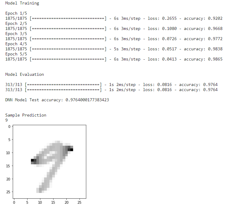
DNN Model Prediction
RNN (LSTM) Model Prediction
The approach for RNN (LSTM) and DNN is the same for the model.
if __name__ == "__main__":
  # load data
  x_train, y_train, x_test, y_test = load_data_NN()
  # load model
  model = RNN(x_train.shape[1:])
  print("nnModel Trainingn")
  model.fit(x_train, y_train, epochs = 5)
  print("nnModel Evaluationn")
  model.evaluate(x_test, y_test)
  score2 = model.evaluate(x_test, y_test, verbose=1)
  print('n''RNN (LSTM) Model Test accuracy:', score2[1])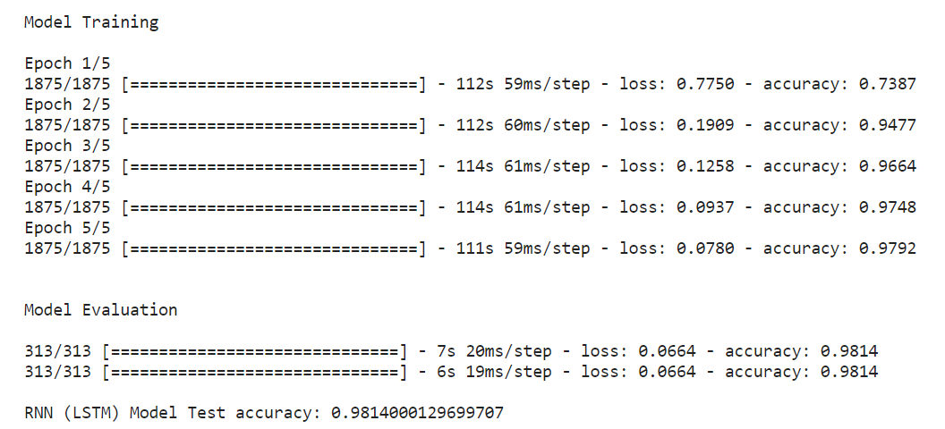
RNN (LSTM) Model Prediction
CNN Model Prediction
For CNN, we will load the load_data_CNN() function; the CNN function differs from the other two because it has a convolution layer, dense, flattening, etc. Along with the train and test set, it has different sizes too. This tailor-made function is beneficial for CNN.
if __name__ == "__main__":
  # load data
  x_train, y_train, x_test, y_test = load_data_CNN()
  # load model
  input_shape = (28,28,1)
  model = CNN(input_shape)
  print("nnModel Trainingn")
  model.fit(x_train, y_train, epochs = 5)
  print("nnModel Evaluationn")
  model.evaluate(x_test, y_test)
  score3 = model.evaluate(x_test, y_test, verbose=1)
  print('n''CNN Model Test accuracy:', score3[1])
  print("nnSample Prediction")
  sample_prediction(20)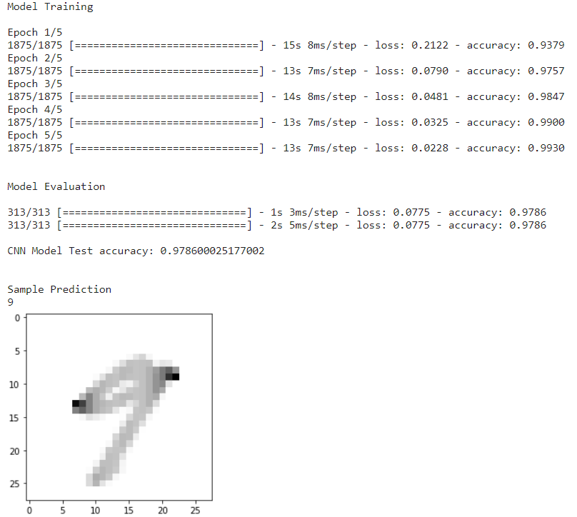
CNN Model Prediction
Once loading the CNN function, the next is to fit the model with 5 epochs. After that model evaluation and test, accuracy is acquired, and will give a sample input image for predicting the image.
Comparing Model Accuracies
After implementing three models and acquiring their scores, comparing them is a must to reach a final statement. The below-mentioned code will present a table format stating the models from best to least accuracies.
The code states, calling the models and their accuracies in an array format, sorting them in descending order, and displaying the output in table format.
results=pd.DataFrame({'Model':['DNN','RNN (LSTM)','CNN'],
                     'Accuracy Score':[score1[1],score2[1],score3[1]]})
result_df=results.sort_values(by='Accuracy Score', ascending=False)
result_df=result_df.set_index('Model')
result_df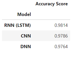
Model accuracies table
The table generated above states that the RNN (LSTM) leads the prediction with a maximum accuracy score, while the CNN is in 2nd place and DNN has the least accuracy score.
What are the steps to creating and training deep learning models?
- Gather data: Collect relevant information for your task, like images for picture recognition.
- Clean and prep: Make sure the data, such as scaling images, are tidy and ready for the model.
- Build a model: Choose the right model architecture based on your task, like a neural network for images.
- Train the model: Show it lots of data and let it learn how to make predictions (like recognizing cats in pictures.
- Evaluate the model: Test it on new data and see how well it does, like how accurate it is at recognizing cats.
- Make predictions: Use the trained model to predict new data, such as identifying new cat pictures.
Conclusion
To summarize the entire execution:
- We imported libraries. Explored and loaded the dataset by plotting a few of the images.
- Then we defined two tailored made functions for DNN, RNN (LSTM), and CNN.
- We implemented algorithms for each of the Deep Learning models.
- After that, we began with the prediction phase for all the Deep Learning models.
- Lastly, we made a comparison table to know which deep learning models are suitable for MNIST dataset prediction.
So, the RNN (LSTM) model is the winner in the entire implementation, scoring 98.54 %. The CNN model got 2nd place with 98.08%, and the DNN model is in 3rd place with 97.21 %. With the final comparison table, the key takeaways are:
- With fast implementation time, the CNN model requires fewer parameters for training, and model performance is maintained.
- With faster execution, the DNN model requires the most parameters for training, but the model performance is compromised with less accuracy.
- With the slowest execution time, the LSTM performed better than the other two. This benefits the LSTM to show better performance.
- Hence, with the above implementation, we can conclude the LSTM model is appropriate for Deep Learning to work with MNIST and other image datasets.
Hopefully, this article helps you to understand how to select appropriate Deep Learning models. Thanks.
Frequently Asked Questions
Modeling in deep learning is like teaching computers to learn from examples. It helps them recognize patterns, make predictions, and understand data.
Deep learning models are used to solve complex tasks like image recognition and language understanding. They improve with experience, making them valuable for various applications
Ethical concerns involve ensuring fairness, preventing biases, protecting privacy, and being transparent about decisions. Responsible use is crucial.
Deep learning models need diverse and representative data for effective learning. More data means better predictions, helping the models understand various scenarios.
The media shown in this article is not owned by Analytics Vidhya and is used at the Author’s discretion.


