Introduction
Often while working on predictive modeling, it is a common observation that most of the time model has good accuracy for the training data and lesser accuracy for the test data. While this is a usual observation for most machine learning problem statements, if the difference between the training and test accuracy is large, it means that the model is overfitting the training data.
There can be multiple reasons for overfitting–
- The model has learned patterns from the random noise in the training data.
- The training and test data are from different time periods. e.g., imagine that you are building a model to identify credit card fraud. Training data has transactions from 2000 to 2019, and Test data contains transactions that happened in 2020 and 2021.
- The training and test data are having different feature values. e.g., Imagine that you are building a model to predict retail sales. Training data contains transactions in European countries, and Test data contains transactions in Asian countries.
If you create the training and test data yourself – you can control and minimize such instances.

However, when you participate in a hackathon, you are usually given 2 datasets – training and test dataset. If the hackathon involves supervised learning, you will also have the training data labels but not the test data.
It may happen that the training data are from different time periods or have different feature values. In such situations, if you build a model using training data and apply it to test data, you may see an accuracy gap between the datasets.
One will say that we can use cross-validation to prevent such gaps. However, cross-validation will take examples or samples from the training data, and this issue will persist.
So, we need to use some other way to identify such trends. Here comes adversarial validation to help us.
This article was published as a part of the Data Science Blogathon.
Table of Contents
What is Adversarial Validation?
Adversarial Validation is a smart yet simple method to identify the similarities between the training and the test dataset. It uses a simple logic – If a binary classifier model is able to differentiate between training and test samples, it means that there is a dissimilarity between the training and the test data.
It involves below basic operations:
- Here, we drop the actual target column from the training dataset.
- Create a label column in both datasets (0 for the train data and 1 for the test data or vice versa).
- Then we combine the training and the test dataset.
- Now, we use a binary classifier to see if we are able to differentiate between the training and test samples.
- Now, we evaluate the AUC ROC score, i.e., the Area Under the Curve for Receiver Operating Characteristic Graph.
If the AUC ROC score is ~0.5, it means that the test and training data are similar.
If the AUC ROC score is >0.5, it means that the test and training data are not similar.
Adversarial Validation in Action
Module 1: Identifying if test and train datasets are similar.
1. Download Dataset and import libraries
We will download the titanic dataset from here.
import pandas as pd
from sklearn.ensemble import RandomForestClassifier
2. Load only numeric features
Python Code:
import pandas as pd
from sklearn.ensemble import RandomForestClassifier
train_data = pd.read_csv("train.csv")
test_data  = pd.read_csv("test.csv")

# select only the numerical features
X_test  = test_data.select_dtypes(include=['number']).copy()
X_train = train_data.select_dtypes(include=['number']).copy()
# drop the target column from the training data
X_train = X_train.drop(['Survived'], axis=1)

print(X_train.shape)
print(X_test.shape)


# add the train/test labels
X_train["Adv_Val_label"] = 0
X_test["Adv_Val_label"]  = 1
# make one big dataset
all_data = pd.concat([X_train, X_test], axis=0, ignore_index=True)

# shuffle
all_data = all_data.sample(frac=1)
forest = RandomForestClassifier(random_state=42,max_depth=2,class_weight='balanced')

X = all_data.drop(['Adv_Val_label'], axis=1).fillna(-1)
y = all_data['Adv_Val_label']

clf = RandomForestClassifier(random_state=42).fit(X, y)
from sklearn.metrics import roc_auc_score
auc_score = roc_auc_score(y, clf.predict_proba(X)[:,1])
print(auc_score)
feature_imp_random_forest = pd.DataFrame({
    'Feature':list(X.columns),
    'RF_Score':list(clf.feature_importances_)
})
feature_imp_random_forest = feature_imp_random_forest.sort_values(by='RF_Score',ascending=False)

feature_imp_random_forest

train_data = pd.read_csv("train.csv")
test_data  = pd.read_csv("test.csv")

# select only the numerical features
X_test  = test_data.select_dtypes(include=['number']).copy()
X_train = train_data.select_dtypes(include=['number']).copy()

# drop the target column from the training data
X_train = X_train.drop(['Survived','PassengerId'], axis=1)
X_test = X_test.drop(['PassengerId'], axis=1)

# add the train/test labels
X_train["Adv_Val_label"] = 0
X_test["Adv_Val_label"]  = 1

# make one big dataset
all_data = pd.concat([X_train, X_test], axis=0, ignore_index=True)

# shuffle
all_data = all_data.sample(frac=1)

X = all_data.drop(['Adv_Val_label'], axis=1).fillna(-1)
y = all_data['Adv_Val_label']

clf = RandomForestClassifier(random_state=42,max_depth=2,class_weight='balanced').fit(X, y)


feature_imp_random_forest = pd.DataFrame({
    'Feature':list(X.columns),
    'RF_Score':list(clf.feature_importances_)
})
feature_imp_random_forest = feature_imp_random_forest.sort_values(by='RF_Score',ascending=False)
feature_imp_random_forest

# Take prob and identify most similar instances to test data
X_new = X.copy()
X_new['proba'] = clf.predict_proba(X)[:,1]
X_new['target'] = y

X_new = X_new[X_new['target']==0]

nrows = X_new.shape[0]
adversarial_validation_data = X_new.sort_values(by='proba',ascending=False)[:int(nrows*.2)]
adversarial_training_data = X_new.sort_values(by='proba',ascending=False)[int(nrows*.2):]
print(adversarial_validation_data)
print(adversarial_training_data)
3. Drop the target feature and create a label column (0 for the train data and 1 for the test data).
# drop the target column from the training data
X_train = X_train.drop(['Survived'], axis=1)

print(X_train.shape)
print(X_test.shape)

# add the train/test labels
X_train["Adv_Val_label"] = 0
X_test["Adv_Val_label"]  = 1
4. Concatenate and shuffle the data
# make one big dataset
all_data = pd.concat([X_train, X_test], axis=0, ignore_index=True)

# shuffle
all_data = all_data.sample(frac=1)
5. Train a Random Forest Model
forest = RandomForestClassifier(random_state=42,max_depth=2,class_weight='balanced')

X = all_data.drop(['Adv_Val_label'], axis=1).fillna(-1)
y = all_data['Adv_Val_label']

clf = RandomForestClassifier(random_state=42).fit(X, y)
6. Look at the roc-auc and Investigate
from sklearn.metrics import roc_auc_score
auc_score = roc_auc_score(y, clf.predict_proba(X)[:,1])
print(auc_score)
Output: 1.0
Here, the ROC score is 1. This means that the model is able to differentiate between the training and test samples completely.
Let us also look at the Feature Importance of feature. This will help to understand which features are driving the predictions.
feature_imp_random_forest = pd.DataFrame({
    'Feature':list(X.columns),
    'RF_Score':list(clf.feature_importances_)
})
feature_imp_random_forest = feature_imp_random_forest.sort_values(by='RF_Score',ascending=False)
feature_imp_random_forest
Upon looking at the Feature Importance, we see that ~97.5% of the importance is due to the PassengerId column.
Let us remove that column and retrain the model.
7. Remove the column and retrain
train_data = pd.read_csv("train.csv")
test_data  = pd.read_csv("test.csv")

# select only the numerical features
X_test  = test_data.select_dtypes(include=['number']).copy()
X_train = train_data.select_dtypes(include=['number']).copy()

# drop the target column from the training data
X_train = X_train.drop(['Survived','PassengerId'], axis=1)
X_test = X_test.drop(['PassengerId'], axis=1)

# add the train/test labels
X_train["Adv_Val_label"] = 0
X_test["Adv_Val_label"]  = 1

# make one big dataset
all_data = pd.concat([X_train, X_test], axis=0, ignore_index=True)

# shuffle
all_data = all_data.sample(frac=1)

X = all_data.drop(['Adv_Val_label'], axis=1).fillna(-1)
y = all_data['Adv_Val_label']

clf = RandomForestClassifier(random_state=42,max_depth=2,class_weight='balanced').fit(X, y)

auc_score = roc_auc_score(y, clf.predict_proba(X)[:,1])
print(auc_score)
Output: 0.6214792797727406
Now for the same hyper-parameters, the ROC score is ~0.62
The score has reduced, making it harder for the model to distinguish between the training and test datasets. Let us also look at the Feature Importance of features. This will help to understand which features are driving the predictions
feature_imp_random_forest = pd.DataFrame({
    'Feature':list(X.columns),
    'RF_Score':list(clf.feature_importances_)
})
feature_imp_random_forest = feature_imp_random_forest.sort_values(by='RF_Score',ascending=False)
feature_imp_random_forest
Output:
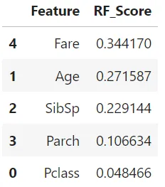
The most important feature is Fare (having ~34.4% importance), followed by Age (having ~27.2% importance), and so on. The feature importance is not biased, unlike the previous run.
Now let us understand how to handle the case when the train and test data differ.
Module 2: How to create a better validation set – when the test and train datasets are different
Here, we will use the same dataset and the model we created in Step 7. Since the ROC score is ~0.62, it means that the test and training data are not similar. So, we need to create a validation set from the original training data that is most similar to the test data. Let us call it adversarial_validation_data
Step 1: The model in step 7 can be used to predict the probability of being a test sample.
# Take prob and identify most similar instances to test data
X_new = X.copy()
X_new['proba'] = clf.predict_proba(X)[:,1]
X_new['target'] = y
Step 2: Remove the original test dataset from this data.
X_new = X_new[X_new['target']==0]Step 3: Sort the data in descending order of probability and pick the top 20% of samples. This would mean that we are selecting samples from the data that are more similar to the test data. Let us call it adversarial_validation_data, and the remaining data will be adversarial_training_data.
nrows = X_new.shape[0]
adversarial_validation_data = X_new.sort_values(by='proba',ascending=False)[:int(nrows*.2)]
adversarial_training_data = X_new.sort_values(by='proba',ascending=False)[int(nrows*.2):]
Now, we can train a machine learning model using adversarial_training_data and optimize its accuracy on the adversarial_validation_data. Your accuracy on adversarial_validation_data will be closer to the actual test data.
Conclusion
Adversarial Validation is a clever and simple method for determining whether our test data and training data are similar; we combine our training and test data, labeling them with a 0 for the training data and a 1 for the test data, mix them up, and then see if we can correctly re-identify them using a binary classifier. In this article,
- we saw how to tackle overfitting and improve the leaderboard scores in a hackathon using adversarial validation.
- We first saw how adversarial validation helps identify whether the test and train datasets are similar or not.
- We also saw how to create a better validation set in case the test and train data differ.
Feel free to connect with me on LinkedIn if you want to discuss this with me.
The media shown in this article is not owned by Analytics Vidhya and is used at the Author’s discretion.
Data Scientist with extensive experience in solving many real world business problems across different domains. Possess fine blend of business knowledge, maths/stats and technology/programming.
Experienced in handling client facing roles, stakeholder management, effective communication with presentation & negotiation skills.


