Covariate Shift – Unearthing hidden problems in Real World Data Science

Introduction

You may have heard from various people that data science competitions are a good way to learn data science, but they are not as useful in solving real world data science problems. Why do you think this is the case?

One of the differences lies in the quality of data that has been provided. In Data Science Competitions, the datasets are carefully curated. Usually, a single large dataset is split into train and test file. So, most of the times the train and test have been generated from the same distribution.

But this is not the case when dealing with real world problems, especially when the data has been collected over a long period of time. In such cases, there may be multiple variables / environment changes might have happened during that period. If proper care is not taken then, the training dataset cannot be used to predict anything about the test dataset in a usable manner.

In this article, we will see the different types of problems or Dataset Shift that we might encounter in the real world. Specifically, we will be talking in detail about one particular kind of shift in the Dataset (Covariate shift), the existing methods to deal with this kind of shift and an in depth demonstration of a particular method to correct this shift.

1. What is Dataset Shift?

Every time you participate in a competition, your journey will look quite similar to the one shown in the figure below.

Let me explain this with the help of a scenario depicted in the picture below. You are given a train and a test file in a competition. You complete the preprocessing, the feature engineering and the cross validation part on the model created but you do not get the same result as the one you get on the cross-validation. No matter what validation strategy you try, it seems like you are bound to get different results in comparison to the cross validation.

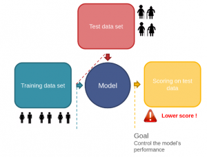
Image source: link

What can be a possible reason for this failure? So, if you carefully notice the first picture, you will find that you did all the manipulation by just looking at the train file. Therefore, you completely ignored the information contained in the test file.

Now take a look back on the second picture, you will notice that the training file contains information about male and females of fairly younger age while the test file contains information about people of older age. Therefore it means that the distribution of data contained in the train and test file is significantly different.

So, if you build your model based on the data set containing information about people having lower age and predict on a data set containing higher values of age, that will definitely give you a low score. The reason is that there will a wide gap in the interest and the activities between these two groups. So your model will fail in these conditions.

This change in the distribution of data contained in train and test file is called dataset shift (or drifting).

2. What causes Dataset Shift?

Try to think some of the examples, where you can encounter the problem of dataset shift.

Basically, in the real world, dataset shift mainly occurs because of the change of environments (popularly called as non-stationary environment), where the environment can be referred as location, time, etc.

Let us consider an example. We collected the sales of various item during the period of July-September. Now your job is to predict the sales during the period of Diwali. The visual representation of sales in the train (blue line) and test (black line) file would be similar to the image shown below.

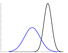
Image source: link

Clearly, the sales during the time of Diwali would be much higher as compared to routine days. Therefore we can say that it is the situation of dataset shift, which occurred due to change of time period between our train and test file.

But our machine learning algorithms work by ignoring these changes. They presume that the train and test environments match and even if they don’t, it assumes that it makes no difference if the environment changes.

Now take a look back at both of the examples that we discussed above. Is there any difference between them?

Yes, in the first scenario, there was a shift in the age (independent variable or predictor) of the population due to which we were getting wrong predictions. While in the latter one, there was a shift in the sales (target variable) of the items. This brings the next topic to the table – Different types of Dataset shifts.

3. Types of Dataset Shift

Dataset shift could be divided into three types:

1. Shift in the independent variables (Covariate Shift)
2. Shift in the target variable (Prior probability shift)
3. Shift in the relationship between the independent and the target variable (Concept Shift)

In this article, we will discuss only covariate shift in this article since the other two topics are still an active research area and there has not been any substantial work to mitigate these problems.

We will also see the methods to identify Covariate shift and the proper measures that can be taken in order to improve the predictions.

4. Covariate Shift

Covariate shift refers to the change in the distribution of the input variables present in the training and the test data. It is the most common type of shift and it is now gaining more attention as nearly every real-world dataset suffers from this problem.

First, let us try to understand how does the change in distribution creates a problem for us. Take a look at the image shown below.

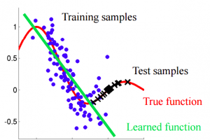
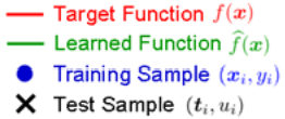
Image source: link

If you carefully notice the image given above, our learning function tries to fit the training data. But here, we can see that the distribution of training and test is different, so predicting using this learned function will definitely give us wrong predictions.

So our first step should be to identify this shift in the distribution. Let’s try and understand it.

5. Identification

Here, I have used a quick and dirty machine learning technique to check whether there is a shift between the training data and the test data.

For this purpose, I will use Sberbank Russian Housing Market dataset from Kaggle.

The basic idea to identify shift – If there exists a shift in the dataset, then on mixing the train and test file, you should still be able to classify an instance of the mixed dataset as train or test with reasonable accuracy. Why?

Because, if the features in both the dataset belong to different distributions then, they should be able to separate the dataset into train and test file significantly.

Let’s try to make it simple. Take a look at the distribution of the feature ‘id’ in both the dataset.

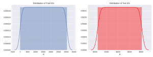
By looking at their distribution, we can clearly see that after a certain value (=30,473), all the instances will belong to test dataset.

So if we create a dataset which is a mixture of training and test instances, where we have labelled each instance of training data as ‘training’ and test as ‘test’ before mixing.

In this new dataset, if we just look at the feature ‘id’, we can clearly classify any instance that whether it belongs to training data or test data. Therefore, we can conclude that ‘id’ is a drifting feature for this dataset.

So this was fairly easy. But we can’t visualise every variable and check whether it is drifting or not. For that purpose, let us try to code this in Python as a simple classification problem and identify the drifting features.

Steps to identify drift

The basic steps that we will follow are:

1. Preprocessing: This step involves imputing all missing values and label encoding of all categorical variables.
2. Creating a random sample of your training and test data separately and adding a new feature origin which has value train or test depending on whether the observation comes from the training dataset or the test dataset.
3. Now combine these random samples into a single dataset. Note that the shape of both the samples of training and test dataset should be nearly equal, otherwise it can be a case of an unbalanced dataset.
4. Now create a model taking one feature at a time while having ‘origin’ as the target variable on a part of the dataset (say ~75%).
5. Now predict on the rest part(~25%) of the dataset and calculate the value of AUC-ROC.
6. Now if the value of AUC-ROC for a particular feature is greater than 0.80, we classify that feature as drifting.

Note that we generally take 0.80 as the threshold value, but the value can be altered based on the situation.

So that is enough of theory, now let’s code this and find which of the features are drifting in this problem.

## importing libraries
import numpy as np
import pandas as pd
from pandas import Series, DataFrame
import os
import warnings
warnings.filterwarnings('ignore')
import matplotlib.pyplot as plt
#get_ipython().magic('matplotlib inline')

from sklearn.ensemble import RandomForestRegressor
from sklearn.ensemble import RandomForestClassifier
from sklearn.model_selection import cross_val_score
from sklearn.preprocessing import LabelEncoder

## reading files
train = pd.read_csv('train_russian_market.csv')
test = pd.read_csv('test_russian_market.csv')

#### preprocessing ####

## missing values
for i in train.columns:
    if train[i].dtype == 'object':
        train[i] = train[i].fillna(train[i].mode().iloc[0])
    if (train[i].dtype == 'int' or train[i].dtype == 'float'):
        train[i] = train[i].fillna(np.mean(train[i]))

for i in test.columns:
    if test[i].dtype == 'object':
        test[i] = test[i].fillna(test[i].mode().iloc[0])
    if (test[i].dtype == 'int' or test[i].dtype == 'float'):
        test[i] = test[i].fillna(np.mean(test[i]))

## label encoding
number = LabelEncoder()
for i in train.columns:
    if (train[i].dtype == 'object'):
        train[i] = number.fit_transform(train[i].astype('str'))
        train[i] = train[i].astype('object')

for i in test.columns:
    if (test[i].dtype == 'object'):
        test[i] = number.fit_transform(test[i].astype('str'))
        test[i] = test[i].astype('object')

## creating a new feature origin
train['origin'] = 0
test['origin'] = 1

training = train.drop('price_doc',axis=1) #droping target variable

## taking sample from training and test data
training = training.sample(7662, random_state=12)
testing = test.sample(7000, random_state=11)

## combining random samples
combi = training.append(testing)
y = combi['origin']
combi.drop('origin',axis=1,inplace=True)

## modelling
model = RandomForestClassifier(n_estimators = 50, max_depth = 5,min_samples_leaf = 5)
drop_list = []
for i in combi.columns:
    score = cross_val_score(model,pd.DataFrame(combi[i]),y,cv=2,scoring='roc_auc')
    if (np.mean(score) > 0.8):
        drop_list.append(i)
        print(i,np.mean(score))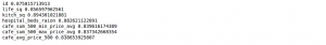

# Drifting features : {id, life_sq, kitch_sq, hospital_beds_raion, cafe_sum_500_min_price_avg, cafe_sum_500_max_price_avg, cafe_avg_price_500 }

Here we have classified seven features as drifting. You can also manually check their difference in distribution through some visualisation or by using 1-way ANOVA test.

So, now the important question is how to treat them effectively such that we can improve our predictions.

6. Treatment

There are different techniques by which we can treat these features in order to improve our model. Let us discuss some of them.

1. Dropping of drifting features
2. Importance weight using Density Ratio Estimation

So let’s try to understand them.

6.1 Dropping

This method is quite simple, as in this, we basically drop the features which are being classified as drifting. But just give it a thought, that simply dropping features might result in some loss of information.

To deal with this, we have defined a simple rule.

Features having a drift value greater than 0.8 and are not important in our model, we drop them.

So, let’s try this in our problem.

Here, I have used a basic random forest model just to check which features are important.

# using a basic model with all the features
training = train.drop('origin',axis=1)
testing = test.drop('origin',axis=1)

rf = RandomForestRegressor(n_estimators=200, max_depth=6,max_features=10)
rf.fit(training.drop('price_doc',axis=1),training['price_doc'])
pred = rf.predict(testing)
columns = ['price_doc']
sub = pd.DataFrame(data=pred,columns=columns)
sub['id'] = test['id']
sub = sub[['id','price_doc']]
sub.to_csv('with_drifting.csv', index=False)

On submitting this file on Kaggle, we are getting a rmse score of 0.40116 on private leaderboard.

So, let’s check first 20 important features for this model.

### plotting importances
features = training.drop('price_doc',axis=1).columns.values
imp = rf.feature_importances_
indices = np.argsort(imp)[::-1][:20]

#plot
plt.figure(figsize=(8,5))
plt.bar(range(len(indices)), imp[indices], color = 'b', align='center')
plt.xticks(range(len(indices)), features[indices], rotation='vertical')
plt.xlim([-1,len(indices)])
plt.show()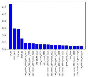

Now, if we compare our drop list and feature importance, we will find that the features ‘life_sq’ and ‘kitch_sq’ are common.

So, we will keep these two features in our model, while dropping the rest of the drifting features.

NOTE: Before dropping any feature, just make sure you if there any possibility to create a new feature from it.

Let’s try this and check whether it improves our prediction or not.

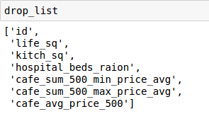
## dropping drifting features which are not important.
drift_train = training.drop(['id','hospital_beds_raion','cafe_sum_500_min_price_avg','cafe_sum_500_max_price_avg','cafe_avg_price_500'], axis=1)
drift_test = testing.drop(['id','hospital_beds_raion','cafe_sum_500_min_price_avg','cafe_sum_500_max_price_avg','cafe_avg_price_500'], axis=1)

rf = RandomForestRegressor(n_estimators=200, max_depth=6,max_features=10)
rf.fit(drift_train.drop('price_doc',axis=1),training['price_doc'])
pred = rf.predict(drift_test)
columns = ['price_doc']
sub = pd.DataFrame(data=pred,columns=columns)
sub['id'] = test['id']
sub = sub[['id','price_doc']]
sub.to_csv('without_drifting.csv', index=False)

On submission of this file on Kaggle, we got a rmse score of 0.39759 on the private leaderboard.

Congratulations, we have successfully improved our performance using this technique.

6.2 Importance weight using Density Ratio Estimation

In this method, the approach to importance estimation would be to first estimate the training and test densities separately and then estimate the importance by taking the ratio of the estimated densities of test and train.

Then these densities act as weights for each instance in the training data.

But giving weights to each instance based on the density ratio could be a rigorous task in higher dimensional data sets. I tried this method on an i7 processor with 128 GB RAM and it took around 3 minutes to calculate the ratio density for a single feature. Also, I could not find any improvement in the score on applying the weights to the training data.

Also scaling this feature for 200 features would be a very time-consuming task.

Therefore, this method is only good up to research papers but the application of this in the real world is still questionable. Also, this is an active area of research.

Conclusion

In summary, Dataset Shift occurs when training and testing data vary, caused by factors like Covariate Shift. Recognizing and addressing these shifts are vital. Steps include identifying drift and applying treatments such as data exclusion or adjusting weights using Density Ratio Estimation.

I hope that now you have a better understanding about drift, how you can identify it and treat it effectively. It has now become a common problem in real world dataset. So you should develop a habit to check this every time while solving problems, and surely it will give you positive results.

Did you find this article helpful? Please share your opinions/thoughts in the comments section below.

FAQs

shubham.jain