Advanced NumPy: Broadcasting and Strides

Introduction

Table of Contents

1. Python For Loops v/s NumPy Vectorization
2. Advanced NumPy: Broadcasting and its Rules
3. Understanding Broadcasting Rules Through Examples
4. Practical Example – Understanding Broadcasting in Image Thresholding
5. Broadcasting and Strides in NumPy
6. Effect of Stride on Cache Performance
7. Conclusion

Python For Loops v/s NumPy Vectorization

If we want to apply an operation to each item of a python list, one straightforward way to do so is using a for a loop. However, if we know that all the elements of the list will be of the same data type, then using a ndarray will prove more beneficial since the time to complete the whole operation will be much less.

This is because, in python, operations on numpy arrays are several times faster when compared to the python list:

1. ndarray (n-dimensional array in numpy) consists of homogeneous elements, while python lists are heterogeneous (containing different datatypes) in nature. This implies that while iterating over each ndarray element, no unnecessary time is spent determining its datatype, which happens in a list.
2. Also, since the elements will be stored in contiguous locations in the memory due to data homogeneity, the locality of reference leads to faster access to these data.
3. Numpy is primarily written in C, which is faster as compared to native python. Thus by doing all the work in C, we gain performance benefits.

However, much of the optimization comes from numpy using vectorized instructions to perform array operations. As mentioned before, it refers to working on the entire array simultaneously rather than on individual elements. Vectorization in the general scope means using SIMD (single instruction multiple data) instruction, i.e., carrying out the same operation on multiple operands in parallel. For example, for adding a scalar and an array, the array can be broken up into chunks, and the CPU can add the scalar to these chunks in parallel. Numpy implements these SIMD functions in the form of ufuncs (Universal functions). Apart from this, numpy performs a lot of other optimizations as well, resulting in faster code.

Advanced NumPy: Broadcasting and its Rules

Broadcasting provides a means for vectorizing the array operations so that looping would take place in C. It is a mechanism used by Numpy when it has to perform arithmetic operations on arrays with different shapes. Usual numpy operations on two arrays are done on an element-by-element basis. However, for this, the arrays must be of the same size. Broadcasting eases this constraint in cases when the shapes of arrays are compatible. So what do we mean by that?
Broadcasting employs the following rules to determine the compatibility of arrays and transform both arrays to the same shape for ease of operations:

1. If the rank (number of dimensions of a numpy array) of two arrays is different
   1.1 A new dimension of size 1 is added to the leftmost side of the array with lesser dimensions (or to the array of lesser rank)
2. Numpy compares dimensions from right to left. When comparing two dimensions
   2.1 If the sizes do not match, then the dimension of size 1 is stretched to the size of the other dimension
   2.2 If neither of the dimension is 1, then the array is deemed incompatible, and broadcasting cannot take place.

Understanding Broadcasting Rules Through Examples

Let’s start with the case when the rank of arrays is the same, i.e., both arrays have the same number of dimensions. The shapes of these arrays are
a: (3,1,5)
b: (1,4,5)
When we compare right to the left, we realize that the third position is the same in both – 5. The second position differs, thus, according to rule 2.1, dimension 1 of a is stretched to 4 to match that of b. Next, moving on to the first position, dimension 1 of b is stretched to 3, thus matching a. The resulting dimension would be (3,4,5). Let’s verify this:

The output to the above code snippet is True.

Now let’s see the arrays with unequal ranks:
a: (3,4,5,6)
b: (5,6)
To compare the above two arrays, we will follow rule 1 and first make their rank equal by prepending 1s to b until its rank becomes equal to
a: (3,4,5,6)
b: (1,1,5,6)
Now we can compare as before. The fourth and third positions are equal. For the second position, 1 of b is stretched to 4; for the first position, 1 of b is stretched to 3. Thus, the overall result should have dimensions as (3,4,5,6). We can verify this by the following code snippet

The above code also results in True.

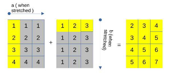
Let’s visualize a broadcasting scenario where both arrays will get stretched. Here, we will make a a column vector with dimensions (4,1) and b as a row vector with dimensions (1,3).

a: (4, 1)
b: (1, 3)
According to our broadcasting rules, dimension 1 of a gets stretched to 3 to match b‘s second dimension, and dimension 1 of b gets stretched to 4 to match a‘s first dimension. This will look like this:

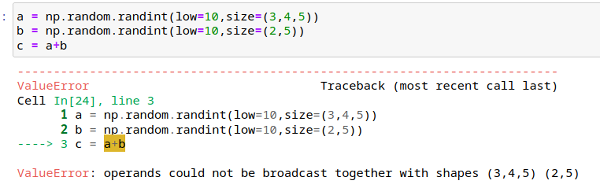
Let’s take a look at one incompatible case now.
a: (3,4,5)
b: (2,5)
Here, we will prepend 1 to b, as before, and thus the dimensions become
a: (3,4,5)
b: (1,2,5)
When we start comparing, we find that the second position differs, and none is 1. Hence, according to rule 2.2, these arrays are incompatible, and broadcasting cannot occur.

The error is shown in the screenshot below:

  
a = np.random.randint(low=10, size = (3,4,5))
b = np.random.randint(low=10, size = (2,5))
c = a+b

Practical Example: Understanding Broadcasting in Image Thresholding

Let’s see broadcasting in action by performing a thresholding operation on an image.

Here, broadcasting comes into play when the array gets multiplied by the scalar 255 in the threshold function.

Broadcasting and Strides in NumPy

To quote from numpy documentation: “Broadcasting provides a means of vectorizing array operations so that looping occurs in C instead of Python. It does this without making needless copies of data and usually leads to efficient algorithm implementations.”
But you would ask: how does it not make copies of data when it is essentially stretching dimensions? And the answer would be strides. Numpy changes the metadata around the arrays, which acts as a means of representing an array bigger than it actually is.
Let’s understand what I mean by that:
Numpy arrays have two major components:

• Raw array data, better known as a data buffer, contains the actual elements stored in our array in a contiguous manner
• Metadata, providing insight as to how we should interpret the data buffer

Let’s see some of the metadata information by defining a function as follows:

As shown above, various metadata about an array includes shape, size, stride, flags, and much more. The interpretation of the data buffer depends on the stride. Dimensions of stride will always be the same as the number of dimensions of an array. In the physical memory, the data is stored in a contiguous format (1- dimensional format), as shown in figure 6 for arr.
Each element occupies 8 bytes (64 bits) of memory for our case since the data type is int64.

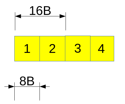
For each dimension, stride represents how many bytes we have to skip to get to the next element of that dimension. For example: for arr, the first row begins at element 1, and the second begins at element 3. So, to get to 3 from 1, we have to skip 16B in the memory. That is why the first element of stride is 16. Similarly, to get the next column value from 1, we need to skip 8B and we will reach 2. Therefore the second element of stride is 8. This makes our stride as (16, 8).

Let’s see what happens when we take the transpose of this array.

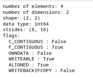
Figure 9: Important metadata about transpose of arr

If we look at the stride information now, we see that the stride dimensions are reversed. But please note that the underlying data buffer has not changed. Numpy did not change the order of the elements in the data buffer. Only the stride information changed meaning that this transpose operation produced a view of the original data buffer.
This can be confirmed as follows:
Hence, we were able to use the same data buffer and interpret data in two different arrays.
Let’s take another example wherein we want to repeat a row vector 3 times. We will use the as_strided function from the stride_tricks library of numpy and provide shape and stride arguments as follows:

Figure 12: Array manipulation using strides

The new interpretation can be understood by noticing that only 8B of data needs to be skipped to move to the next column element. However, to fetch data for the new row, we are still going to use the existing row, and therefore the stride value is 0.
Thus, internally, array broadcasting is implemented using 0 strides. Let’s implement broadcasting through strides by taking an example of the element-wise addition of two arrays – a, a row vector, and b, a column vector.

In the above example, we will make a row vector and b column vector. Thus a will have shape (1,4) and b will have shape (3,1). Now, let’s apply the broadcasting rules that we learned earlier and see what should be the dimensions of our result:
a: (1,4)
b: (3,1)
Going from right to left, 1 of b will be stretched to become 4, and then next, 1 of a will be stretched to become 3. Thus, the result will have dimensions (3,4).

Figure 16: Code output for the addition of a1 and b1

As we can see above, we were able to implement broadcasting using the 0-stride mechanism. Using only 3 elements of b, we were able to represent an array of 12 elements in b1. This is why we can use strides to represent virtually larger arrays with a relatively small data buffer.
However, we must be careful when using strides. This is because some operations, such as np.copy, might copy the full array size, thus rendering our efforts useless.

Effect of Stride on Cache Performance

Our memory layout greatly affects performance in numpy. Since the CPU fetches data from memory in blocks and caches it, if our strides are smaller such that array item that is required consecutively comes in one block, then our operations would be faster since fewer transfers will be required in and out of the cache. Thus, smaller strides might result in better performance overall.

Conclusion

To conclude, NumPy provides a flexible and optimized framework for the scientific computations of large and higher dimensional arrays. Vectorization is the reason behind the efficiency of numpy. Following are our key takeaways from this article:

1. Vectorization is the application of an operation to an entire array at once.
2. Broadcasting acts as means of vectorizing array operations by checking the compatibility of array shapes.
3. Broadcasting rules work as though the smaller dimensions get stretched to bigger ones if arrays are compatible.
4. The internal makeup of a numpy array involves strides. Stride in a dimension refers to the number of bytes required to skip to reach the next element in that particular dimension.
5. Internally, broadcasting is implemented through 0-strides.
6. A smaller stride often translates to better cache performance.

The media shown in this article is not owned by Analytics Vidhya and is used at the Author’s discretion.