Using GANs in TensorFlow Generate Images

Introduction

In this article, we explore the application of GANs in TensorFlow for generating unique renditions of handwritten digits. The GAN framework comprises two key components: the generator and the discriminator. The generator generates new images in a randomized manner, whereas the discriminator is designed to differentiate between authentic and counterfeit images. Through GAN training, we obtain a collection of images that closely resemble handwritten digits. The primary objective of this article is to outline the procedure for constructing and evaluating GANs using the MNIST dataset.

Learning Objectives

1. This article provides a comprehensive introduction to Generative Adversarial Networks (GANs) and explores their applications in image generation.
2. The main objective of this tutorial is to guide readers through the step-by-step process of constructing a GAN using the TensorFlow library. It covers training the GAN on the MNIST dataset to generate new images of handwritten digits.
3. The article discusses the architecture and components of GANs, including generators and discriminators, to enhance readers’ understanding of their fundamental workings.
4. To aid learning, the article includes code examples that demonstrate various tasks, such as reading and preprocessing the MNIST dataset, building the GAN architecture, calculating loss functions, training the network, and evaluating the results.
5. Furthermore, the article explores the expected outcome of GANs, which is a collection of images that bear a striking resemblance to handwritten digits.

This article was published as a part of the Data Science Blogathon.

What are we building?

Generating novel images using preexisting image databases is a prominent feature of specialized models called Generative Adversarial Networks (GANs). GANs excel in producing unsupervised or semi-supervised images leveraging diverse image datasets.

This article harnesses the image-generation potential of GANs to create handwritten digits. The methodology entails training the network on a handwritten digit database. In this instructional piece, we will construct a rudimentary GAN utilizing the Tensorflow library, conduct training on the MNIST dataset, and generate fresh images of handwritten digits.

How do we set this up?

The primary emphasis of this article revolves around harnessing the image generation potential of GANs. The procedure commences with the loading and preprocessing of the image database to facilitate the GAN training process. Once the data is successfully loaded, we proceed to construct the GAN model and develop the necessary code for training and testing. In the subsequent section, detailed instructions are provided on implementing this functionality and generating a fresh image using the MNIST database.

Model Building

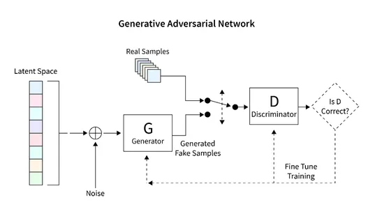
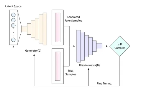
The GAN model we aim to build consists of two important components:

• Generator: This component is responsible for generating new images.
• Discriminator: This component evaluates the quality of the generated image.

The general architecture that we will develop to generate images using GAN is shown in the diagram below. The following section provides a brief description of how to read the database, create the required architecture, calculate the loss function, and train the network. Additionally, code is provided to inspect the network and generate new images.

Reading the Dataset

The MNIST dataset holds great prominence in the field of computer vision and comprises a vast collection of handwritten digits with dimensions of 28×28 pixels. This dataset proves to be ideal for our GAN implementation due to its grayscale, single-channel image format.

The subsequent code snippet demonstrates the utilization of a built-in function in Tensorflow to load the MNIST dataset. Upon successful loading, we proceed to normalize and reshape the images into a three-dimensional format. This transformation enables efficient processing of the 2D image data within the GAN architecture. Additionally, memory is allocated for both training and validation data.

The shape of each image is defined as a 28x28x1 matrix, where the last dimension represents the number of channels in the image. As the MNIST dataset comprises grayscale images, we only have a single channel.

In this particular instance, we set the size of the latent space, denoted as “zsize,” to 100. This value can be adjusted according to specific requirements or preferences.

from __future__ import print_function, division
from keras.datasets import mnist
from keras.layers import Input, Dense, Reshape, Flatten, Dropout
from keras.layers import BatchNormalization, Activation, ZeroPadding2D
from keras.layers import LeakyReLU
from keras.layers.convolutional import UpSampling2D, Conv2D
from keras.models import Sequential, Model
from keras.optimizers import Adam, SGD
import matplotlib.pyplot as plt
import sys
import numpy as np

num_rows = 28
num_cols = 28
num_channels = 1
input_shape = (num_rows, num_cols, num_channels)
z_size = 100

(train_ims, _), (_, _) = mnist.load_data()
train_ims = train_ims / 127.5 - 1.
train_ims = np.expand_dims(train_ims, axis=3)

valid = np.ones((batch_size, 1))
fake = np.zeros((batch_size, 1))

Defining the Generator

The Generator (D) assumes a crucial role in GANs as it is responsible for generating realistic images that can deceive the discriminator. It serves as the primary component for image formation in GANs. In this study, we utilize a specific architecture for the Generator, which incorporates a fully connected (FC) layer and employs Leaky ReLU activation. However, it is worth noting that the last layer of the Generator utilizes TanH activation instead of LeakyReLU. This adjustment was made to ensure that the generated image resides within the same interval (-1, 1) as the original MNIST database.

def build_generator():
    gen_model = Sequential()
    gen_model.add(Dense(256, input_dim=z_size))
    gen_model.add(LeakyReLU(alpha=0.2))
    gen_model.add(BatchNormalization(momentum=0.8))
    gen_model.add(Dense(512))
    gen_model.add(LeakyReLU(alpha=0.2))
    gen_model.add(BatchNormalization(momentum=0.8))
    gen_model.add(Dense(1024))
    gen_model.add(LeakyReLU(alpha=0.2))
    gen_model.add(BatchNormalization(momentum=0.8))
    gen_model.add(Dense(np.prod(input_shape), activation='tanh'))
    gen_model.add(Reshape(input_shape))

    gen_noise = Input(shape=(z_size,))
    gen_img = gen_model(gen_noise)
    return Model(gen_noise, gen_img)

Defining the Discriminator

In a Generative Adversarial Network (GAN), the Discriminator (D) performs the critical task of differentiating between real images and generated images by assessing their authenticity and likelihood. This component can be seen as a binary classification problem. To address this task, we can employ a simplified network architecture comprising Fully Connected Layers (FC), Leaky ReLU activation, and Dropout Layers. It is important to mention that the final layer of the Discriminator includes an FC layer followed by Sigmoid activation. The Sigmoid activation function produces the desired classification probability.

def build_discriminator():
    disc_model = Sequential()
    disc_model.add(Flatten(input_shape=input_shape))
    disc_model.add(Dense(512))
    disc_model.add(LeakyReLU(alpha=0.2))
    disc_model.add(Dense(256))
    disc_model.add(LeakyReLU(alpha=0.2))
    disc_model.add(Dense(1, activation='sigmoid'))

    disc_img = Input(shape=input_shape)
    validity = disc_model(disc_img)
    return Model(disc_img, validity)

Computing the Loss Function

In order to ensure a good image generation process in GANs, it is important to determine the appropriate metrics to evaluate its performance. Define this parameter by the loss function.

The discriminator is responsible for dividing the generated image into real or fake and giving the probability of being real. To achieve this difference, the Discriminator aims to maximize the function D(x) when presented with a real image and minimize D(G(z)) when presented with a false image.

On the other hand, the purpose of the Generator is to fool the Discriminator by creating a realistic image that can be misinterpreted. Mathematically, this involves scaling D(G(z)). However, only relying on this component as a loss function can cause the network to be overconfident with wrong results. To solve this problem, we use the log of the loss function (D(G(z)).

The overall cost function of the GAN to generate an image can be expressed as a minimal game:

min_G max_D V(D,G) = E(xp_data(x))(log(D(x))] + E(zp(z))(log(1 – D(G(z)))])

Such GAN training requires a fine balance and can take as a match between two opponents. Each side seeks to influence and outdo the other by playing the MinMax game.

We can use Binary Cross Entropy Loss to implement Generator and Discriminator.

For the implementation of the Generator and Discriminator, we can utilize the Binary Cross entropy loss.

# discriminator
disc= build_discriminator()
disc.compile(loss='binary_crossentropy',
    optimizer='sgd',
    metrics=['accuracy'])

z = Input(shape=(z_size,))

# generator
img = generator(z)

disc.trainable = False

validity = disc(img)

# combined model
combined = Model(z, validity)
combined.compile(loss='binary_crossentropy', optimizer='sgd')

Optimizing the Loss

To facilitate the training of the network, our objective is to involve the GAN in a MinMax game. This learning process revolves around optimizing the network weights through the use of Gradient Descent. In order to accelerate the learning process and prevent convergence to suboptimal loss landscapes, Stochastic Gradient Descent (SGD) is employed.

Given that the Discriminator and Generator have distinct losses, a single loss function cannot simultaneously optimize both systems. Consequently, utlize the separate loss functions for each system.

def intialize_model():
    disc= build_discriminator()
    disc.compile(loss='binary_crossentropy',
        optimizer='sgd',
        metrics=['accuracy'])

    generator = build_generator()

    z = Input(shape=(z_size,))
    img = generator(z)

    disc.trainable = False

    validity = disc(img)

    combined = Model(z, validity)
    combined.compile(loss='binary_crossentropy', optimizer='sgd')
    return disc, Generator, and combined

After specifying all the required features, we can train the system and optimize the loss. The steps to train a GAN to generate an image are as follows:

• Load the image and generate a random sound of the same size as the loaded image.
• Differentiate between the uploaded image and the sound produced and consider the possibility of real or fake.
• Produce another random noise of the same magnitude and provide as input to the generator.
• Train the generator for a specific period.
• Repeat these steps until the image is satisfactory.

def train(epochs, batch_size=128, sample_interval=50):
    # load images
    (train_ims, _), (_, _) = mnist.load_data()
    # preprocess
    train_ims = train_ims / 127.5 - 1.
    train_ims = np.expand_dims(train_ims, axis=3)

    valid = np.ones((batch_size, 1))
    fake = np.zeros((batch_size, 1))
    # training loop
    for epoch in range(epochs):

        batch_index = np.random.randint(0, train_ims.shape[0], batch_size)
        imgs = train_ims[batch_index]
    # create noise
        noise = np.random.normal(0, 1, (batch_size, z_size))
    # predict using a Generator
        gen_imgs = gen.predict(noise)
    # calculate loss functions
        real_disc_loss = disc.train_on_batch(imgs, valid)
        fake_disc_loss = disc.train_on_batch(gen_imgs, fake)
        disc_loss_total = 0.5 * np.add(real_disc_loss, fake_disc_loss)

        noise = np.random.normal(0, 1, (batch_size, z_size))

        g_loss = full_model.train_on_batch(noise, valid)
   
    # save outputs every few epochs
        if epoch % sample_interval == 0:
            one_batch(epoch)

Generating Handwritten Digits

Using the MNIST dataset, we can create a utility function to generate predictions for a set of images using the Generator. This function generates a random sound, supply it to the generator, run it to display the generated image and saves it in a special folder. Recommend to run this utility function periodically, such as every 200 cycles, to monitor network progress. The implementation is below:

def one_batch(epoch):
    r, c = 5, 5
    noise_model = np.random.normal(0, 1, (r * c, z_size))
    gen_images = gen.predict(noise_model)

    # Rescale images 0 - 1
    gen_images = gen_images*(0.5) + 0.5

    fig, axs = plt.subplots(r, c)
    cnt = 0
    for i in range(r):
        for j in range(c):
            axs[i,j].imshow(gen_images[cnt, :,:,0], cmap='gray')
            axs[i,j].axis('off')
            cnt += 1
    fig.savefig("images/%d.png" % epoch)
    plt.close()

In our experiment, we trained the GAN for approximately 10,000 epochs using a batch size of 32. To track the progress of the training, we saved the generated images every 200 epochs and stored them in a designated folder called “images.”

disc, gen, full_model = intialize_model()
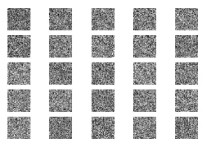
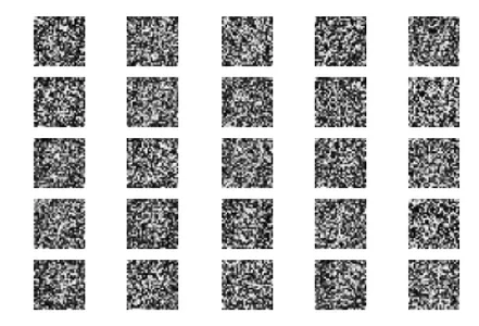
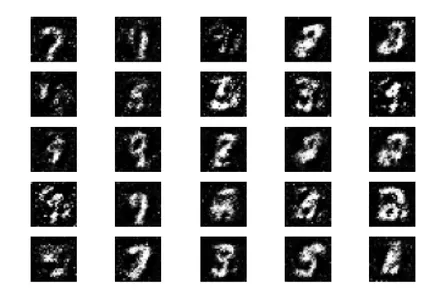
train(epochs=10000, batch_size=32, sample_interval=200)

Now, let’s examine the GAN simulation results at different stages: initialization, 400 epochs, 5000 epochs, and the final result at 10000 epochs.

Initially, we start with random noise as the input to the Generator.

After 400 epochs of training, we can observe some progress, although the generated images still differ significantly from real digits.

After training for 5000 epochs, we can observe that the generated figures start to resemble the MNIST dataset.

Complete the full 10,000 epochs of training, we obtain the following outputs.

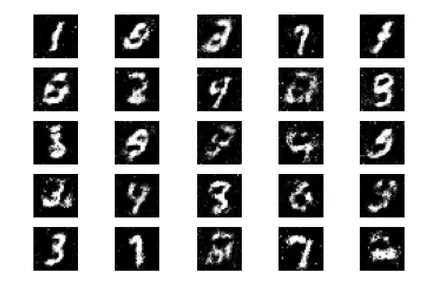
These generated images closely resemble the handwritten number data to train the network. It is important to note that these images are not part of the training set and entirely generated by the network.

Next Steps

Now that we have achieved good results in GAN’s image generation, there are many ways we can further improve it. Within the scope of this discussion, we may consider experimenting with different parameters. Here are a few suggestions:

• Explore different values ​​for the latent space variable z_size to see if it increases efficiency.
• Increase the number of training epochs to over 10,000. Doubling or tripling the duration of training may reveal improved or degraded results.
• Try using different datasets like fashion MNIST or moving MNIST. Since these datasets have the same structure as MNIST, adapt our existing code.
• Consider experimenting with alternative architectures such as CycleGun, DCGAN, and others. Modifying the generator and discriminator functions may be sufficient to explore these models.

By implementing these changes, we can further enhance the capabilities of GANs and explore new possibilities in image generation.

These generated images closely resemble the handwritten number data that uses to train the network. These images are not part of the training set and generated entirely by the network.

Conclusion

In summary, GAN is a powerful machine learning model capable of generating new images based on existing databases. In this tutorial, we have shown how to design and train a simple GAN using the Tensorflow library as an example and the MNIST database.

Key Takeaways

• GAN consists of two important components: a generator, which is responsible for generating new images from random input, and the Discriminator, which aims to distinguish between real and fake images.
• Through the learning process, we have succeeded in creating a set of images that closely resemble handwritten digits, as shown in the example image.
• To optimize GAN performance, we provide matching metrics and loss functions that help distinguish real and fake images. By evaluating GANs on unseen data and using Generators, we can generate new, previously unseen images.
• Overall, GANs offer interesting possibilities in image generation and have great potential for several applications such as machine learning and computer vision.

Frequently Asked Questions

The media shown in this article is not owned by Analytics Vidhya and is used at the Author’s discretion.

ANURAG SINGH CHOUDHARY 12 Jul 2023