MNIST Dataset Prediction Using Keras!

This article was published as a part of the Data Science Blogathon

Introduction:

This blog deals with MNIST Data. Actually, MNIST is ‘Modified National Institute of Standards and Technology. This dataset consists of handwritten digits from 0 to 9 and it provides a pavement for testing image processing systems. This is considered to be the ‘hello world program in Machine Learning’ which involves Deep Learning.

Steps Involved are:

1.  Importing Dataset
2.  Split the Dataset into Test and Train
3.  Model Building
4.  Train the Model
5. Predicting the Accuracy

1) Importing Dataset:

To proceed further with the code we need the dataset. So, we think about various sources like datasets, UCI, kaggle, etc. But since we are using Python with its vast inbuilt modules it has the MNIST Data in the keras.datasets module. So, we don’t need to externally download and store the data.

from keras.datsets import mnist
data = mnist.load_data()

Therefore from keras.datasets module we import the mnist function which contains the dataset.

Then the data set is stored in the variable data using the mnist.load_data() function which loads the dataset into the variable data.

Next, let’s see the data type we find something unusual as it of the type tuple. We know that the mnist dataset contains handwritten digit images, stored in the form of tuples.

data
type(data)

2) Split the Dataset into Train and Test:

We directly split the dataset into train and test. So for that, we initialize four variables X_train, y_train, X_test, y_test to sore the train and test data of dependent and independent values respectively.

(X_train, y_train), (X_test, y_test) = data
X_train[0].shape
X_train.shape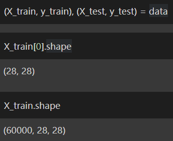

While printing the shape of each image we can find that it is 28×28 in size. Meaning the image has 28pixels x 28pixels.

Now, we have to reshape in such a way that we have we can access every pixel of the image. The reason to access every pixel is that only then we can apply deep learning ideas and can assign color code to every pixel. Then we store the reshaped array in X_train, X_test respectively.

X_train = X_train.reshape((X_train.shape[0], 28*28)).astype('float32')
X_test = X_test.reshape((X_test.shape[0], 28*28)).astype('float32')

We know the RGB color code where different values produce various colors. It is also difficult to remember every color combination. So, refer to this link to get a brief idea about RGB Color Codes.

We already know that each pixel has its unique color code and also we know that it has a maximum value of 255. To perform Machine Learning, it is important to convert all the values from 0 to 255 for every pixel to a range of values from 0 to 1. The simplest way is to divide the value of every pixel by 255 to get the values in the range of 0 to 1.

X_train = X_train / 255
X_test = X_test / 255

Now we are done with splitting the data into test and train as well as making the data ready for further use. Therefore, we can now move to Step 3: Model Building.

3) Train the Model:

To perform Model building we have to import the required functions i.e. Sequential and Dense to execute Deep Learning which is available under the Keras library.

But this is not directly available for which we need to understand this simple line chart:

1) Keras -> Models -> Sequential

2) Keras -> Layers -> Dense

Let’s see the way we can import the functions with the same logic as a python code.

from keras.models import Sequential
from keras.layers import Dense
model = Sequential()
model.add(Dense(32, input_dim = 28 * 28, activation= 'relu'))
model.add(Dense(64, activation = 'relu'))
model.add(Dense(10, activation = 'softmax'))

Then we store the function in the variable model as it makes it easier to access the function every time instead of typing the function every time, we can use the variable and call the function.

Then convert the image into a dense pool of layers and stack each layer one above the other and we use ‘relu’ as our activation function. The explanation of ‘relu’ is beyond the scope of this blog. To learn more about it you can refer to it.

Then again, we stack a few more layers with ‘softmax’ as our activation function. To learn more about ‘softmax’ function you can refer to this article as it is beyond this blog’s scope again as my primary aim is to get the highest possible accuracy with the MNIST Data Set.

Then finally we compile the entire model and use cross-entropy as our loss function, to optimize our model use adam as our optimizer and use accuracy as our metrics to evaluate our model.

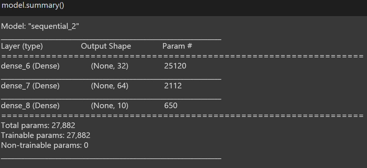
To get an overview of our model we use ‘model.summary()’, which provides brief details about our model.

Now we can move to Step 4: Train the Model.

4) Train the Model:

This is the penultimate step where we are going to train the model with just a single line of code. So for that, we are using the .fit() function which takes the train set of the dependent and the independent and dependent variable as the input, and set epochs = 10, and set batch_size as 100.

Train set => X_train; y_train

Epochs => An epoch means training the neural network with all the training data for one cycle. An epoch is made up of one or more batches, where we use a part of the dataset to train the neural network. Meaning we send the model to train 10 times to get high accuracy. You could also change the number of epochs depending on how the model performs.

Batch_size => Batch size is a term used in machine learning and refers to the number of training examples utilized in one iteration. So basically, we send 100 images to train as a batch per iteration.

Let’s see the coding part of it.

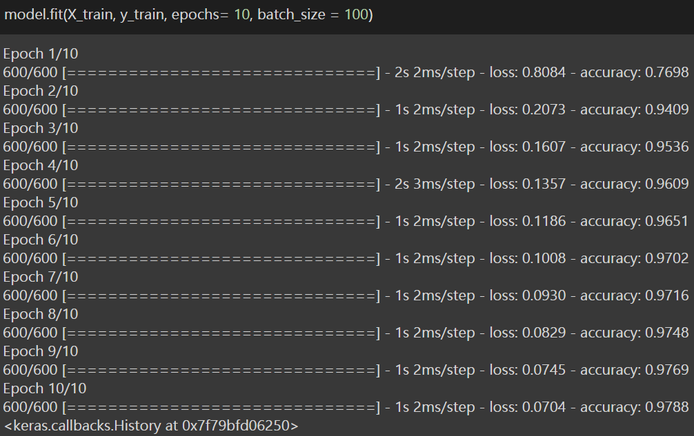
Hence, after training the model we have achieved an accuracy of 97.88% for the training data set. Now, it’s time to see how the model works in the test set and see whether we have achieved the required accuracy. Therefore, we now move on to the ultimate step or Step 5: Predicting Accuracy.

5) Predicting Accuracy:

So to know how well the model works in the testing dataset I use the scores variable to store the value and use the .evaluate() function which takes the test set of the dependent and the independent variables as the input. This computes the loss and the accuracy of the model in the test set. As we are focused on accuracy we print only the accuracy.

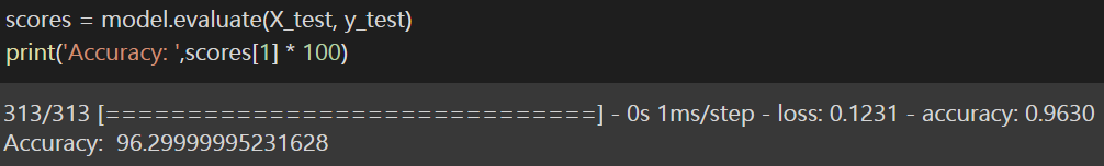
Finally, we have achieved the result and we secured an accuracy of more than 96% in the test set which is very much appreciable, and the motive of the blog is achieved. I have scripted the link to the notebook for your(readers) reference.

Please feel free to connect with me through Linkedin as well. And thanks for reading the blog.

The media shown in this article are not owned by Analytics Vidhya and are used at the Author’s discretion.