Introduction

Agriculture has always been a cornerstone of human civilization, providing sustenance and livelihoods for billions worldwide. As technology advances, we find new and innovative ways to enhance agricultural practices. One such advancement is using Vision Transformers (ViTs) to classify leaf diseases in crops. In this blog, we’ll explore how vision transformers in agriculture revolutionize by offering an efficient and accurate solution for identifying and mitigating crop diseases.

Cassava, or manioc or yuca, is a versatile crop with various uses, from providing dietary staples to industrial applications. Its hardiness and resilience make it an essential crop for regions with challenging growing conditions. However, cassava plants are vulnerable to various diseases, with CMD and CBSD being among the most destructive.

CMD is caused by a complex of viruses transmitted by whiteflies, leading to severe mosaic symptoms on cassava leaves. CBSD, on the other hand, is caused by two related viruses and primarily affects storage roots, rendering them inedible. Identifying these diseases early is crucial for preventing widespread crop damage and ensuring food security. Vision Transformers, an evolution of the transformer architecture initially designed for natural language processing (NLP), have proven highly effective in processing visual data. These models process images as sequences of patches, using self-attention mechanisms to capture intricate patterns and relationships in the data. In the context of cassava leaf disease classification, ViTs are trained to identify CMD and CBSD by analyzing images of infected cassava leaves.

Learning Outcomes

• Understanding Vision Transformers and how they are applied to agriculture, specifically for leaf disease classification.
• Learn about the fundamental concepts of the transformer architecture, including self-attention mechanisms, and how these are adapted for visual data processing.
• Understand the innovative use of Vision Transformers (ViTs) in agriculture, specifically for the early detection of cassava leaf diseases.
• Gain insights into the advantages of Vision Transformers, such as scalability and global context, as well as their challenges, including computational requirements and data efficiency.

This article was published as a part of the Data Science Blogathon.

The Rise of Vision Transformers

Computer vision has made tremendous strides in recent years, thanks to the development of convolutional neural networks (CNNs). CNNs have been the go-to architecture for various image-related tasks, from image classification to object detection. However, Vision Transformers have risen as a strong alternative, offering a novel approach to processing visual information. Researchers at Google Research introduced Vision Transformers in 2020 in a groundbreaking paper titled “An Image is Worth 16×16 Words: Transformers for Image Recognition at Scale.” They adapted the transformer architecture, initially designed for natural language processing (NLP), to the domain of computer vision. This adaptation has opened up new possibilities and challenges in the field.

The use of ViTs offers several advantages over traditional methods, including:

• High Accuracy: ViTs excel in accuracy, allowing for the reliable detection and differentiation of leaf diseases.
• Efficiency: Once trained, ViTs can process images quickly, making them suitable for real-time disease detection in the field.
• Scalability: ViTs can handle datasets of varying sizes, making them adaptable to different agricultural settings.
• Generalization: ViTs can generalize to different cassava varieties and disease types, reducing the need for specific models for each scenario.

The Transformer Architecture: A Brief Overview

Before diving into Vision Transformers, it’s essential to understand the core concepts of the transformer architecture. Transformers, originally designed for NLP, revolutionized language processing tasks. The key features of transformers are self-attention mechanisms and parallelization, allowing for more comprehensive context understanding and faster training.

At the heart of transformers is the self-attention mechanism, which enables the model to weigh the importance of different input elements when making predictions. This mechanism, combined with multi-head attention layers, captures complex relationships in data.

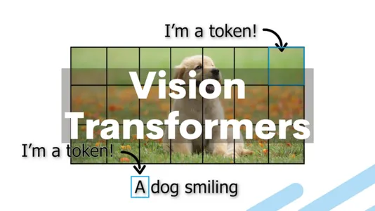
So, how do Vision Transformers apply this transformer architecture to the domain of computer vision? The fundamental idea behind Vision Transformers is to treat an image as a sequence of patches, just as NLP tasks treat text as a sequence of words. The transformer layers then process each patch in the image by embedding it into a vector.

Key Components of a Vision Transformer

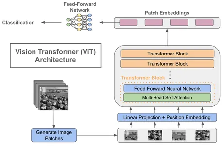
• Patch Embeddings: Divide an image into fixed-size, non-overlapping patches, typically 16×16 pixels. Each patch is then linearly embedded into a lower-dimensional vector.
• Positional Encodings: Add Positional encodings to the patch embeddings to account for the spatial arrangement of patches. This allows the model to learn the relative positions of patches within the image.
• Transformer Encoder: Vision Transformers consist of multiple transformer encoder layers like NLP transformers. Each layer performs self-attention and feed-forward operations on the patch embeddings.
• Classification Head: At the end of the transformer layers, a classification head is added for tasks like image classification. It takes the output embeddings and produces class probabilities.

The introduction of Vision Transformers marks a significant departure from CNNs, which rely on convolutional layers for feature extraction. By treating images as sequences of patches, Vision Transformers achieve state-of-the-art results in various computer vision tasks, including image classification, object detection, and even video analysis.

Implementation

Dataset

The Cassava Leaf Disease dataset comprises around 15,000 high-resolution images of cassava leaves exhibiting various stages and degrees of disease symptoms. Each image is meticulously labeled to indicate the disease present, allowing for supervised machine learning and image classification tasks. Cassava diseases exhibit distinct characteristics, leading to their classification into several categories. These categories include Cassava Bacterial Blight (CBB), Cassava Brown Streak Disease (CBSD), Cassava Green Mottle (CGM), and Cassava Mosaic Disease (CMD). Researchers and data scientists leverage this dataset to train and evaluate machine learning models, including deep neural networks like Vision Transformers (ViTs).

Importing the Necessary Libraries

import numpy as np
import pandas as pd
import tensorflow as tf
import tensorflow.keras.layers as L
import tensorflow_addons as tfa
import glob, random, os, warnings
import matplotlib.pyplot as plt
from sklearn.metrics import confusion_matrix, classification_report
import seaborn as sns csv

Load the Dataset

image_size = 224
batch_size = 16
n_classes = 5

train_path = '/kaggle/input/cassava-leaf-disease-classification/train_images'
test_path = '/kaggle/input/cassava-leaf-disease-classification/test_images'

df_train = pd.read_csv('/kaggle/input/cassava-leaf-disease-classification/train.csv', dtype = 'str')

test_images = glob.glob(test_path + '/*.jpg')
df_test = pd.DataFrame(test_images, columns = ['image_path'])

classes = {0 : "Cassava Bacterial Blight (CBB)",
           1 : "Cassava Brown Streak Disease (CBSD)",
           2 : "Cassava Green Mottle (CGM)",
           3 : "Cassava Mosaic Disease (CMD)",
           4 : "Healthy"}#import csv

Data Augmentation

def data_augment(image):
    p_spatial = tf.random.uniform([], 0, 1.0, dtype = tf.float32)
    p_rotate = tf.random.uniform([], 0, 1.0, dtype = tf.float32)
 
    image = tf.image.random_flip_left_right(image)
    image = tf.image.random_flip_up_down(image)
    
    if p_spatial > .75:
        image = tf.image.transpose(image)
        
    # Rotates
    if p_rotate > .75:
        image = tf.image.rot90(image, k = 3) # rotate 270º
    elif p_rotate > .5:
        image = tf.image.rot90(image, k = 2) # rotate 180º
    elif p_rotate > .25:
        image = tf.image.rot90(image, k = 1) # rotate 90º
        
    return image#import csv

Data Generator

datagen = tf.keras.preprocessing.image.ImageDataGenerator(samplewise_center = True,
                                                          samplewise_std_normalization = True,
                                                          validation_split = 0.2,
                                                          preprocessing_function = data_augment)

train_gen = datagen.flow_from_dataframe(dataframe = df_train,
                                        directory = train_path,
                                        x_col = 'image_id',
                                        y_col = 'label',
                                        subset = 'training',
                                        batch_size = batch_size,
                                        seed = 1,
                                        color_mode = 'rgb',
                                        shuffle = True,
                                        class_mode = 'categorical',
                                        target_size = (image_size, image_size))

valid_gen = datagen.flow_from_dataframe(dataframe = df_train,
                                        directory = train_path,
                                        x_col = 'image_id',
                                        y_col = 'label',
                                        subset = 'validation',
                                        batch_size = batch_size,
                                        seed = 1,
                                        color_mode = 'rgb',
                                        shuffle = False,
                                        class_mode = 'categorical',
                                        target_size = (image_size, image_size))

test_gen = datagen.flow_from_dataframe(dataframe = df_test,
                                       x_col = 'image_path',
                                       y_col = None,
                                       batch_size = batch_size,
                                       seed = 1,
                                       color_mode = 'rgb',
                                       shuffle = False,
                                       class_mode = None,
                                       target_size = (image_size, image_size))#import csv

images = [train_gen[0][0][i] for i in range(16)]
fig, axes = plt.subplots(3, 5, figsize = (10, 10))

axes = axes.flatten()

for img, ax in zip(images, axes):
    ax.imshow(img.reshape(image_size, image_size, 3))
    ax.axis('off')

plt.tight_layout()
plt.show()#import csv

Model Building

learning_rate = 0.001
weight_decay = 0.0001
num_epochs = 1

patch_size = 7  # Size of the patches to be extract from the input images
num_patches = (image_size // patch_size) ** 2
projection_dim = 64
num_heads = 4
transformer_units = [
    projection_dim * 2,
    projection_dim,
]  # Size of the transformer layers
transformer_layers = 8
mlp_head_units = [56, 28]  # Size of the dense layers of the final classifier

def mlp(x, hidden_units, dropout_rate):
    for units in hidden_units:
        x = L.Dense(units, activation = tf.nn.gelu)(x)
        x = L.Dropout(dropout_rate)(x)
    return x

Patch Creation

In our cassava leaf disease classification project, we employ custom layers to facilitate extracting and encoding image patches. These specialized layers are instrumental in preparing our data for processing by the Vision Transformer model.

class Patches(L.Layer):
    def __init__(self, patch_size):
        super(Patches, self).__init__()
        self.patch_size = patch_size

    def call(self, images):
        batch_size = tf.shape(images)[0]
        patches = tf.image.extract_patches(
            images = images,
            sizes = [1, self.patch_size, self.patch_size, 1],
            strides = [1, self.patch_size, self.patch_size, 1],
            rates = [1, 1, 1, 1],
            padding = 'VALID',
        )
        patch_dims = patches.shape[-1]
        patches = tf.reshape(patches, [batch_size, -1, patch_dims])
        return patches
        
plt.figure(figsize=(4, 4))

x = train_gen.next()
image = x[0][0]

plt.imshow(image.astype('uint8'))
plt.axis('off')

resized_image = tf.image.resize(
    tf.convert_to_tensor([image]), size = (image_size, image_size)
)

patches = Patches(patch_size)(resized_image)
print(f'Image size: {image_size} X {image_size}')
print(f'Patch size: {patch_size} X {patch_size}')
print(f'Patches per image: {patches.shape[1]}')
print(f'Elements per patch: {patches.shape[-1]}')

n = int(np.sqrt(patches.shape[1]))
plt.figure(figsize=(4, 4))

for i, patch in enumerate(patches[0]):
    ax = plt.subplot(n, n, i + 1)
    patch_img = tf.reshape(patch, (patch_size, patch_size, 3))
    plt.imshow(patch_img.numpy().astype('uint8'))
    plt.axis('off')
    
class PatchEncoder(L.Layer):
    def __init__(self, num_patches, projection_dim):
        super(PatchEncoder, self).__init__()
        self.num_patches = num_patches
        self.projection = L.Dense(units = projection_dim)
        self.position_embedding = L.Embedding(
            input_dim = num_patches, output_dim = projection_dim
        )

    def call(self, patch):
        positions = tf.range(start = 0, limit = self.num_patches, delta = 1)
        encoded = self.projection(patch) + self.position_embedding(positions)
        return encoded#import csv

Patches Layer (class Patches(L.Layer)

The Patches layer initiates our data preprocessing pipeline by extracting patches from raw input images. These patches represent smaller, non-overlapping regions of the original image. The layer operates on batches of images, extracting specific-sized patches and reshaping them for further processing. This step is essential for enabling the model to focus on fine-grained details within the image, contributing to its ability to capture intricate patterns.

Visualization of Image Patches

Following patch extraction, we visualize their impact on the image by displaying a sample image overlaid with a grid showcasing the extracted patches. This visualization offers insights into how the image is divided into these patches, highlighting the patch size and the number of patches extracted from each image. It aids in understanding the preprocessing stage and sets the stage for subsequent analysis.

Patch Encoding Layer (class PatchEncoder(L.Layer)

Once the patches are extracted, they undergo further processing through the PatchEncoder layer. This layer is pivotal in encoding the information contained within each patch. It consists of two key components: a linear projection that enhances the patch’s features and a position embedding that adds spatial context. The resulting enriched patch representations are critical for the Vision Transformer’s analysis and learning, ultimately contributing to the model’s effectiveness in accurate disease classification.

The custom layers, Patches and PatchEncoder, are integral to our data preprocessing pipeline for cassava leaf disease classification. They enable the model to focus on image patches, enhancing its capacity to discern pertinent patterns and features essential for precise disease classification. This process significantly bolsters the overall performance of our Vision Transformer model.

def vision_transformer():
    inputs = L.Input(shape = (image_size, image_size, 3))
    
    # Create patches.
    patches = Patches(patch_size)(inputs)
    
    # Encode patches.
    encoded_patches = PatchEncoder(num_patches, projection_dim)(patches)

    # Create multiple layers of the Transformer block.
    for _ in range(transformer_layers):
        
        # Layer normalization 1.
        x1 = L.LayerNormalization(epsilon = 1e-6)(encoded_patches)
        
        # Create a multi-head attention layer.
        attention_output = L.MultiHeadAttention(
            num_heads = num_heads, key_dim = projection_dim, dropout = 0.1
        )(x1, x1)
        
        # Skip connection 1.
        x2 = L.Add()([attention_output, encoded_patches])
        
        # Layer normalization 2.
        x3 = L.LayerNormalization(epsilon = 1e-6)(x2)
        
        # MLP.
        x3 = mlp(x3, hidden_units = transformer_units, dropout_rate = 0.1)
        
        # Skip connection 2.
        encoded_patches = L.Add()([x3, x2])

    # Create a [batch_size, projection_dim] tensor.
    representation = L.LayerNormalization(epsilon = 1e-6)(encoded_patches)
    representation = L.Flatten()(representation)
    representation = L.Dropout(0.5)(representation)
    
    # Add MLP.
    features = mlp(representation, hidden_units = mlp_head_units, dropout_rate = 0.5)
    
    # Classify outputs.
    logits = L.Dense(n_classes)(features)
    
    # Create the model.
    model = tf.keras.Model(inputs = inputs, outputs = logits)
    
    return model
    
decay_steps = train_gen.n // train_gen.batch_size
initial_learning_rate = learning_rate

lr_decayed_fn = tf.keras.experimental.CosineDecay(initial_learning_rate, decay_steps)

lr_scheduler = tf.keras.callbacks.LearningRateScheduler(lr_decayed_fn)

optimizer = tf.keras.optimizers.Adam(learning_rate = learning_rate)

model = vision_transformer()
    
model.compile(optimizer = optimizer, 
              loss = tf.keras.losses.CategoricalCrossentropy(label_smoothing = 0.1), 
              metrics = ['accuracy'])


STEP_SIZE_TRAIN = train_gen.n // train_gen.batch_size
STEP_SIZE_VALID = valid_gen.n // valid_gen.batch_size

earlystopping = tf.keras.callbacks.EarlyStopping(monitor = 'val_accuracy',
                                                 min_delta = 1e-4,
                                                 patience = 5,
                                                 mode = 'max',
                                                 restore_best_weights = True,
                                                 verbose = 1)

checkpointer = tf.keras.callbacks.ModelCheckpoint(filepath = './model.hdf5',
                                                  monitor = 'val_accuracy', 
                                                  verbose = 1, 
                                                  save_best_only = True,
                                                  save_weights_only = True,
                                                  mode = 'max')

callbacks = [earlystopping, lr_scheduler, checkpointer]

model.fit(x = train_gen,
          steps_per_epoch = STEP_SIZE_TRAIN,
          validation_data = valid_gen,
          validation_steps = STEP_SIZE_VALID,
          epochs = num_epochs,
          callbacks = callbacks)
#import csv

Code Explanation

This code defines a custom Vision Transformer model tailored for our cassava disease classification task. It encapsulates multiple Transformer blocks, each consisting of multi-head attention layers, skip connections, and multi-layer perceptrons (MLPs). The result is a robust model capable of capturing intricate patterns in cassava leaf images.

Firstly, the vision_transformer() function takes center stage by defining the architectural blueprint of our Vision Transformer. This function outlines how the model processes and learns from cassava leaf images, enabling it to classify diseases precisely.

To further optimize the training process, we implement a learning rate scheduler. This scheduler employs a cosine decay strategy, dynamically adjusting the learning rate as the model learns. This dynamic adaptation enhances the model’s convergence, allowing it to reach its peak performance efficiently.

We proceed with model compilation once our model’s architecture and training strategy are set. During this phase, we specify essential components such as the loss functions, optimizers, and evaluation metrics. These elements are carefully chosen to ensure that our model optimizes its learning process, making accurate predictions.

Finally, the effectiveness of our model’s training is ensured by applying training callbacks. Two critical callbacks come into play: early stopping and model checkpointing. Early stopping monitors the model’s performance on validation data and intervenes when improvements stagnate, thus preventing overfitting. Simultaneously, model checkpointing records the best-performing version of our model, allowing us to preserve its optimal state for future use.

Together, these components create a holistic framework for developing, training, and optimizing our Vision Transformer model, a key step in our journey toward accurate cassava leaf disease classification.

Applications of ViTs in Agriculture

The application of Vision Transformers in cassava farming extends beyond research and novelty; it offers practical solutions to pressing challenges:

• Early Disease Detection: ViTs enable early detection of CMD and CBSD, allowing farmers to take prompt action to prevent the spread of diseases and minimize crop losses.
• Resource Efficiency: With ViTs, resources such as time and use labor more efficiently, as automated disease detection reduces the need for manual inspection of every cassava plant.
• Precision Agriculture: Integrate ViTs with other technologies like drones and IoT devices for precision agriculture, where disease hotspots are identified and treated precisely.
• Improved Food Security: By mitigating the impact of diseases on cassava yields, ViTs contribute to enhanced food security in regions where cassava is a dietary staple.

Advantages of Vision Transformers

Vision Transformers offer several advantages over traditional CNN-based approaches:

• Scalability: Vision Transformers can handle images of varying resolutions without requiring changes to the model architecture. This scalability is particularly valuable in real-world applications where images come in different sizes.
• Global Context: The self-attention mechanism in Vision Transformers allows them to capture global context effectively. This is crucial for tasks like recognizing objects in cluttered scenes.
• Fewer Architectural Components: Unlike CNNs, Vision Transformers do not require complex architectural components like pooling layers and convolutional filters. This simplifies model design and maintenance.
• Transfer Learning: Vision Transformers can be pretrained on large datasets, making them excellent candidates for transfer learning. Pretrained models can be fine-tuned for specific tasks with relatively small amounts of task-specific data.

Challenges and Future Directions

While Vision Transformers have shown remarkable progress, they also face several challenges:

• Computational Resources: Training large Vision Transformer models requires substantial computational resources, which can be a barrier for smaller research teams and organizations.
• Data Efficiency: Vision Transformers can be data-hungry, and achieving robust performance with limited data can be challenging. Developing techniques for more data-efficient training is a pressing concern.
• Interpretability: Transformers are often criticized for their black-box nature. Researchers are working on methods to improve the interpretability of Vision Transformers, especially in safety-critical applications.
• Real-time Inference: Achieving real-time inference with large Vision Transformer models can be computationally intensive. Optimizations for faster inference are an active research area.

Conclusion

Vision Transformers transform cassava farming by offering accurate and efficient solutions for leaf disease classification. Their ability to process visual data, coupled with advancements in data collection and model training, holds tremendous potential for safeguarding cassava crops and ensuring food security. While challenges remain, ongoing research and practical applications drive driving adoption of ViTs in cassava farming. Continued innovation and collaboration will transform ViTs into an invaluable tool for cassava farmers worldwide, as they contribute to sustainable farming practices and reduce crop losses caused by devastating leaf diseases.

Key Takeaways

• Vision Transformers (ViTs) adapt transformer architecture for computer vision, processing images as sequences of patches.
• ViTs, initially designed for computer vision, are now being applied to agriculture to address challenges like the early detection of leaf diseases.
• Address challenges like computational resources and data efficiency, making ViTs a promising technology for the future of computer vision.

Frequently Asked Questions

The media shown in this article is not owned by Analytics Vidhya and is used at the Author’s discretion. 

Shruti Sureshan 12 Oct 2023