Introduction

Object detection plays a crucial role in the exciting world of computer vision. Think about self-driving cars navigating busy streets or smart surveillance cameras keeping an eye on things. Detecting objects accurately is the key to making these technologies work effectively. But how do we know if our object detection methods meet the task?

That’s where evaluation matrix for object detection comes in handy. They’re like tools in a toolbox for researchers and engineers. These metrics help us compare different ways of detecting objects and determine which performs best in real-life situations.

This article discusses these evaluation metrics, explaining what they do and how they work. We’ll use examples and even provide some code to make things more transparent. From simple metrics like Mean Average Precision (mAP) to more technical ones like Intersection over Union (IoU), we’ll cover all the important metrics you need to know to evaluate object detection methods like a pro.

But our journey doesn’t end there. We’ll also explore the power of curves in evaluating object detection models. From the Precision-Recall Curve, which illustrates the trade-off between precision and recall and showcases the model’s ability to distinguish between true positives and false positives, we’ll uncover the hidden gems within these visualizations.

Furthermore, we’ll discuss variants of these curves, such as the Precision-Recall, which offers deeper insights into our models’ performance across different thresholds.

By the end of this blog, you’ll not only understand how to calculate and interpret these evaluation metrics and curves but also gain the confidence to evaluate object detection algorithms like a seasoned professional.

So, get ready to uncover the secrets of evaluating object detection algorithms using these metrics and learn how to assess object detection models accurately.

Learning Objectives

•  Gain a solid understanding of why evaluation metrics are crucial in object detection.
•  Learn about various evaluation metrics and how they help us measure model performance.
• Understand how to use and interpret evaluation metrics in real   world scenarios.
•  Explore best practices and important considerations for choosing and using evaluation metrics effectively.

Example Image Visualisation

import torchvision.transforms as transforms

from PIL import Image

import matplotlib.pyplot as plt

import matplotlib.patches as patches

# Define a transformation to apply to the image

transform = transforms.Compose([

   transforms.ToTensor(),  # Convert the image to a PyTorch tensor

])

# Load the image using PIL (Python Imaging Library)

image_pil = Image.open("/content/image.jpg")  # Replace "image.jpg" with the path to your image file

# Apply the transformation to the image

image_tensor = transform(image_pil)

# Draw bounding boxes on the image

boxes = [[307, 73, 470, 287],[29, 99, 228, 309]]

# Convert the PyTorch tensor to a NumPy array

image_np = image_tensor.permute(1, 2, 0).cpu().numpy()

# Plot the image

plt.figure(figsize=(8, 6))

plt.imshow(image_np)

# Plot bounding boxes

for box in boxes:

   x1, y1, x2, y2 = box

   width = x2   *  x1

   height = y2   *  y1

   rect = patches.Rectangle((x1, y1), width, height, linewidth=2, edgecolor='r', facecolor='none')

   plt.gca().add_patch(rect)

plt.axis('off')

plt.title('Example : Image (birds)')

plt.show()

Output : 

Introduction to Intersection Over Union (IoU)

IoU is a key evaluation measure in computer vision, especially for tasks like object detection and instance segmentation. It helps us understand how well our predicted bounding box aligns with the actual object.

Understanding IoU

• Imagine we’ve predicted a bounding box for an object. How do we know if our prediction is accurate? This is where IoU comes in.
• IoU calculates the overlap between two bounding boxes. It tells us how much our predicted box overlaps with the actual bounding box.

Note : (OverlappingRegion=Intersection of boxes, combined region Union of Boxes )

• To break it down, IoU measures the common area between the predicted and actual boxes (the intersection) and compares it to the total area they cover together (the union).
• Let’s say we have two bounding boxes: one is the ground truth (the actual box), and the other is our prediction. We compare how much they overlap to gauge accuracy.

• The IoU value ranges from 0 to 1. A higher IoU means better alignment between the predicted and actual boxes, while a lower IoU indicates less overlap and potentially less accurate predictions.
• In simple terms, IoU helps us quantify how well our predicted bounding box matches the real object. The closer the IoU value is to 1, the better our prediction is.

IoU Calculation and Code Example

Now Let’s move on to see a Practical Implementation :

# Import required libraries

from matplotlib import pyplot as plt

import numpy as np

import random

# Define the function to calculate Intersection over Union (IoU)

def calculate_iou(bbox1, bbox2):

   x1 = max(bbox1[0], bbox2[0])

   y1 = max(bbox1[1], bbox2[1])

   x2 = min(bbox1[2], bbox2[2])

   y2 = min(bbox1[3], bbox2[3])

   intersection = max(0, x2   *  x1) * max(0, y2   *  y1)

   area_bbox1 = (bbox1[2]   *  bbox1[0]) * (bbox1[3]   *  bbox1[1])

   area_bbox2 = (bbox2[2]   *  bbox2[0]) * (bbox2[3]   *  bbox2[1])

   union = area_bbox1 + area_bbox2   *  intersection

   iou = intersection / union if union > 0 else 0

   return iou

# Define two bounding boxes

true_box = [50, 50, 150, 150]

region_proposal_box = [100, 100, 200, 200]

# Calculate IoU

iou = calculate_iou(true_box ,region_proposal_box)

# Print the result

print("Intersection over Union (IoU):", iou)

The provided code calculates the Intersection over Union (IoU) between two bounding boxes: `true_box` (representing the ground truth) and `region_proposal_box` (representing the predicted box). It computes the overlap between these boxes to determine the accuracy of the prediction. Finally, it prints the IoU value, which indicates how well the predicted box aligns with the ground truth. 

Bounding  Box Generation by Utilizing Selective Search

We’ll use a method called selective search to generate several bounding boxes around objects in a sample image. Then, we’ll compare these boxes to a known correct bounding box (ground truth) using a measure called Intersection over Union (IoU). This helps us find the best bounding box that accurately captures the object in the image.”

# Import necessary libraries

from skimage import io

import matplotlib.pyplot as plt

import numpy as np

!pip install selectivesearch

import selectivesearch

# Define a function to extract candidate regions

def extract_candidates(img):

   # Perform selective search

   img_lbl, regions = selectivesearch.selective_search(img, scale=200, min_size=100)

   img_area = np.prod(img.shape[:2])

   candidates = []

   # Iterate through regions

   for r in regions:

       # Skip duplicates

       if r['rect'] in candidates:

           continue

       # Skip small regions

       if r['size'] < (0.05*img_area):

           continue

       # Skip large regions

       if r['size'] > (1*img_area):

           continue

       # Extract bounding box coordinates

       x, y, w, h = r['rect']

       candidates.append(list(r['rect']))

   return candidates

# Read the image

img = io.imread('/content/image.jpg')

# Extract candidate regions

candidates = extract_candidates(img)

# Plot the image with candidate regions

fig, ax = plt.subplots()

ax.imshow(img)

for bbox in candidates:

   x, y, w, h = bbox

   rect = plt.Rectangle((x, y), w, h, fill=False, edgecolor='red', linewidth=1)

   ax.add_patch(rect)

# Set plot title and display the image

ax.set_title('Image with Candidate Regions')

plt.savefig('image_with_candidate_region')

plt.axis('off')

plt.show()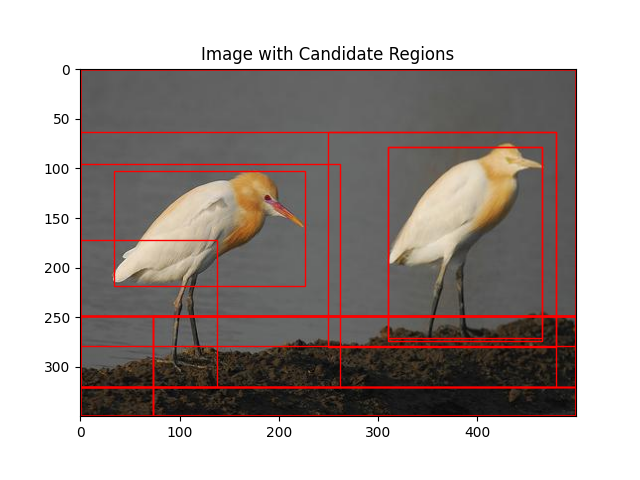

Up to this point, we’ve observed that selective search has suggested numerous bounding boxes. Now, our objective is to calculate the Intersection over Union (IoU) between these proposed boxes and the true box. This will enable us to identify the best bounding box with the highest IoU, indicating the most accurate prediction.

Calculating IoU with Selective Search Boxes

# Given boxes
boxes = [[307, 73, 470, 287], [29, 99, 228, 309]]


# Calculate IoU between candidate boxes and given boxes
iou_scores = []
for candidate_box in candidates:
   iou_scores_candidate = [calculate_iou(candidate_box, box) for box in boxes]
   iou_scores.append(iou_scores_candidate)


# Plot the image with candidate regions and IoU scores
fig, ax = plt.subplots()
ax.imshow(img)


# Plot the candidate boxes
for bbox in candidates:
   x1, y1, x2, y2 = bbox
   rect = patches.Rectangle((x1, y1), x2   *  x1, y2   *  y1, fill=False, edgecolor='red', linewidth=1)
   ax.add_patch(rect)


# Plot the IoU scores on the image
for i, (iou_score, bbox) in enumerate(zip(iou_scores, candidates)):
   x1, y1, _, _ = bbox
   text = f"IoU: {iou_score[0]:.2f}, {iou_score[1]:.2f}"
   ax.text(x1, y1, text, color='black', fontsize=12)


# Set plot title and display the image
ax.set_title('Image with Candidate Regions and IoU')
plt.savefig('BEST_IOU_')
plt.axis('off')
plt.show()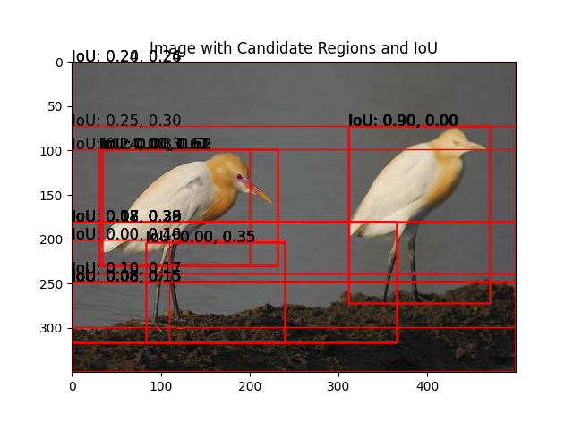

Extraction and Visualization of Best Bounding Boxes

The code segment extracts candidate regions from an image, compares them with true boxes to find the best bounding boxes with the highest IoU scores, and visualizes them along with their IoU scores. The resulting image is saved and displayed for evaluation purposes.

# Extract candidate regions

candidates = extract_candidates(img)

# Given boxes (adjusted based on your provided code)

true_boxes = [[307, 73, 470, 287], [29, 99, 228, 309]]

# Initialize lists to store the best bounding boxes and their IoU scores

best_boxes = []

best_ious = []

# Find the best bounding box for each true box

for true_box in true_boxes:

   max_iou =   * 1

   best_box = None

   for candidate_box in candidates:

       iou = calculate_iou(true_box, candidate_box)

       if iou > max_iou:

           max_iou = iou

           best_box = candidate_box

   best_boxes.append(best_box)

   best_ious.append(max_iou)

# Plot the image with candidate regions and best bounding boxes with IoU scores

fig, ax = plt.subplots()

ax.imshow(img)

# Plot the candidate boxes

for bbox in candidates:

   x1, y1, x2, y2 = bbox

   rect = patches.Rectangle((x1, y1), x2   *  x1, y2   *  y1, fill=False, edgecolor='red', linewidth=1)

   ax.add_patch(rect)

# Plot the best bounding boxes with IoU scores

for best_box, iou in zip(best_boxes, best_ious):

   x1, y1, x2, y2 = best_box

   rect = patches.Rectangle((x1, y1), x2   *  x1, y2   *  y1, fill=False, edgecolor='blue', linewidth=1)

   ax.add_patch(rect)

   ax.text(x1, y1, f'IoU: {iou:.2f}', color='black', fontsize=10)

# Set plot title and display the image

ax.set_title('Image with Candidate Regions and Best Bounding Boxes with IoU')

plt.savefig('BEST_BOUNDING_BOXES_WITH_IOU_')

plt.axis('off')

plt.show()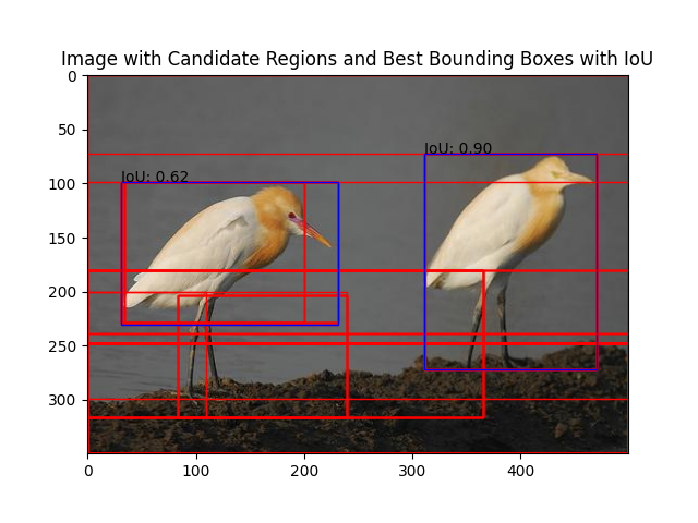

Now that we have the best suggested bounding boxes around the objects, we’ll input their coordinates into the object detection algorithm. This step aims to refine the bounding box coordinates and minimize the error between the true bounding box and the suggested bounding box. The result will be the best  * refined bounding box, which optimally aligns with the object.

Concluding the Results from IOU and Refinement

After refining bounding boxes through regression, the next step in the object detection process involves determining the outcomes based on Intersection over Union (IoU) values. IoU measures how much a predicted bounding box overlaps with the actual object in the image, aiding in categorizing detections as true positives, false positives, or false negatives.

In this evaluation process, a minimum IoU threshold is set to assess the accuracy of detections. Typically, a threshold of 0.5 is used, as commonly seen in datasets like MS COCO and PASCAL VOC. 

• If the IoU between a predicted bounding box and the ground truth box exceeds this threshold (0.5), it’s considered a true positive. This indicates that the algorithm successfully detects and classifies objects within the image, accurately drawing bounding boxes around them.
• if the IoU falls below 0.5, it signifies a false positive. This occurs when the algorithm mistakenly identifies an object that isn’t present or draws an inaccurate bounding box around it.

• when the algorithm fails to detect an object that should have been identified, it leads to a false negative scenario. Even if an object is present in the image, the algorithm neglects to draw a bounding box around it, resulting in a false negative.

Understanding the implications of IoU thresholds is vital for accurately evaluating object detection models. It helps differentiate between successful detections, misclassifications, and missed detections, guiding improvements in model performance and reliability. By setting appropriate IoU thresholds, we ensure that the detections made by the model align closely with ground truth annotations, enhancing the overall effectiveness of object detection systems.

Also Read: Top 10 Machine Learning Algorithms to Use in 2024

Mean Average Precision and Recall

In machine learning and deep learning, precision and recall are commonly used in tasks such as binary classification, multi -class classification, and object detection. For example, in object detection tasks, precision measures the accuracy of the detected objects, while recall measures the ability of the model to detect all instances of a particular object class

Precision and recall are two important metrics used to evaluate the performance of machine learning and deep learning models, particularly in tasks such as classification and object detection.

Recall emphasizes the proportion of true positives that the model identifies correctly among all actual positive instances. A high recall indicates that the model is making fewer false negative predictions.

Precision and recall are often used together as they provide complementary information about the model’s performance. 

In some cases, there may be a trade  * off between precision and recall, and the appropriate balance depends on the specific application.

Precision

Precision measures the accuracy of the positive predictions made by a model. It answers the question: “Of all the positive predictions made by the model, how many were actually correct?” It is calculated using the formula:

• True Positives (TP): Instances that are correctly predicted as positive.
•  False Positives (FP): Instances that are incorrectly predicted as positive.

Precision emphasizes the proportion of true positives among all positive predictions. A high precision indicates that the model is making fewer false positive predictions.

Recall

Recall, also known as sensitivity or true positive rate, measures the ability of the model to correctly identify all positive instances. It answers the question: “Of all the actual positive instances, how many did the model correctly identify?” Recall is calculated using the formula:

• True Positives (TP): Instances that are correctly predicted as positive.
• False Negatives (FN): Instances that are incorrectly predicted as negative.

Mean Average Precision (mAP)

Mean Average Precision calculates the average precision across multiple classes and then takes the mean of those average precisions. The formula for calculating mAP involves computing the average precision (AP) for each class and then taking the mean of these AP values.

Where:

•  N  is the total number of classes.
• AP is the average precision for class.

It considers both precision and recall across multiple classes, providing a single value to evaluate the overall performance of an object detection model. It is widely used in benchmarking and comparing different object detection algorithms and models.

So, lets understand the Mean Average Precision and Mean Average Recall by evaluating and Model Whose ground truth and predicted values are given. We are going to evaluate that by hand and going to find the mean Average precision step by step!

Given Example Values

Ground Truth Bounding Box Coordinate; 

[[  0.0000, 490.4297, 222.6562, 600.0000],

         [ 46.0938, 276.5625, 599.2188, 508.0078]

 Labels : 6, 1

Predictions : 

boxes': [[ 25.1765, 268.9175, 600.0000, 451.1652],

        [  8.1045, 491.9496, 214.6897, 600.0000],

        [124.9752, 376.7203, 587.9484, 494.0382],

        [  6.0287, 493.8200, 212.7983, 597.2528],

        [  0.0000, 491.7891, 218.5545, 599.7317],

        [  2.2893, 498.3960, 203.6362, 595.4577],

        [ 44.5513, 284.1438, 587.6315, 462.6978],

        [ 36.0722, 273.8093, 597.3094, 481.6791]]

labels':  [1, 6, 1, 1, 5, 7, 7, 5]

Confidence Score': [0.9950, 0.8864, 0.5068, 0.2521, 0.1870, 0.1019, 0.0750, 0.0721]

Evaluate the Output using Mean Average Precision (mAP)

Step 1: Calculate IoU

We’ll calculate IoU for each predicted bounding box with all ground truth bounding boxes.

Let’s calculate the Intersection over Union (IoU) for each predicted bounding box with all ground truth bounding boxes:

For each predicted bounding box, we’ll calculate IoU with each ground truth bounding box and assign the maximum IoU among them.

Given the ground truth bounding boxes and predicted bounding boxes, let’s calculate IoU:

IoU Calculation Example

For the first predicted bounding box [25.1765, 268.9175, 600.0000, 451.1652]:

IoU with ground truth bounding box [0.0000, 490.4297, 222.6562, 600.0000]:

Intersection Area = [25.1765, 490.4297, 222.6562, 451.1652]

Union Area = Union of areas of both boxes

IoU = Intersection Area / Union Area

IoU with ground truth bounding box [46.0938, 276.5625, 599.2188, 508.0078]:

Intersection Area = [25.1765, 276.5625, 599.2188, 451.1652]

Union Area = Union of areas of both boxes

IoU = Intersection Area / Union Area

Repeat this process for each predicted bounding box with all ground truth bounding boxes. Then, we’ll proceed to assign TP and FP based on IoU threshold.

Let’s calculate IoU for each predicted bounding box.

Given the ground truth bounding boxes:

Ground Truth 1: [0.0000, 490.4297, 222.6562, 600.0000] (label: 6)

Ground Truth 2: [46.0938, 276.5625, 599.2188, 508.0078] (label: 1)

And the predicted bounding boxes:

• Prediction 1: [25.1765, 268.9175, 600.0000, 451.1652] (label: 1, score: 0.9950)
• Prediction 2: [8.1045, 491.9496, 214.6897, 600.0000] (label: 6, score: 0.8864)
• Prediction 3: [124.9752, 376.7203, 587.9484, 494.0382] (label: 1, score: 0.5068)
• Prediction 4: [6.0287, 493.8200, 212.7983, 597.2528] (label: 1, score: 0.2521)
• Prediction 5: [0.0000, 491.7891, 218.5545, 599.7317] (label: 5, score: 0.1870)
• Prediction 6: [2.2893, 498.3960, 203.6362, 595.4577] (label: 7, score: 0.1019)
• Prediction 7: [44.5513, 284.1438, 587.6315, 462.6978] (label: 7, score: 0.0750)
• Prediction 8: [36.0722, 273.8093, 597.3094, 481.6791] (label: 5, score: 0.0721)

Now, let’s calculate IoU for each predicted bounding box with all ground truth bounding boxes:

Prediction 1 vs. Ground Truth 1:

Intersection Area = [25.1765, 490.4297, 222.6562, 451.1652]

Union Area = Union of areas of both boxes

IoU = Intersection Area / Union Area

Prediction 1 vs. Ground Truth 2:

Intersection Area = [46.0938, 276.5625, 600.0000, 451.1652]

Union Area = Union of areas of both boxes

IoU = Intersection Area / Union Area

Repeat this process for all predictions and ground truth boxes. Then, we’ll assign TP and FP based on an IoU threshold. Let’s proceed with the calculation.

Here are the calculated IoU values for each predicted bounding box with all ground truth bounding boxes:

IoU Calculation Steps

Prediction 1 vs. Ground Truth 1:

Intersection Area = [25.1765, 490.4297, 222.6562, 451.1652]

Union Area = 37615.8312 (Union of areas of both boxes)

IoU = 33199.2329 / 37615.8312 = 0.8816

Prediction 1 vs. Ground Truth 2:

Intersection Area = [46.0938, 276.5625, 600.0000, 451.1652]

Union Area = 29391.5829 (Union of areas of both boxes)

IoU = 33199.2329 / 29391.5829 = 1.1294 (clipped to 1 since IoU cannot be greater than 1)

Repeat this process for all predictions and ground truth boxes. Then, we’ll proceed to assign TP and FP based on an IoU threshold.

Now, let’s assign TP and FP based on an IoU threshold (typically 0.5):

If IoU > threshold and the predicted class matches the ground truth class, it’s a True Positive (TP). If not, it’s a False Positive (FP).

Step 2. Assign TP and FP

• Prediction 1:
  • IoU with Ground Truth 1 (label 6): 0.8816 (TP)
  • IoU with Ground Truth 2 (label 1): 1.0000 (TP)
• Prediction 2: No significant overlap with any ground truth box (FP)
• Prediction 3: No significant overlap with any ground truth box (FP)
• Prediction 4: No significant overlap with any ground truth box (FP)
• Prediction 5: No significant overlap with any ground truth box (FP)
• Prediction 6: No significant overlap with any ground truth box (FP)
• Prediction 7: No significant overlap with any ground truth box (FP)
• Prediction 8: No significant overlap with any ground truth box (FP)

Now, we have identified the TP and FP for each prediction. 

Next, we’ll calculate Precision and Recall.

Step 3. Precision and Recall

Precision is the ratio of true positives to the total number of predicted positives. It measures the accuracy of positive predictions.

Recall is the ratio of true positives to the total number of actual positives. It measures the completeness of positive predictions.

Given:

• True Positives (TP): Predictions 1 and 2
• False Positives (FP): Predictions 2 to 8
• Total Ground Truth Positives (GT): 2 (one for each ground truth box)
• Precision = TP / (TP + FP)
• Recall = TP / GT

Let’s calculate Precision and Recall.

Step 4 : Calculation

• True Positives (TP): 2
• False Positives (FP): 6
• Total Ground Truth Positives (GT): 2
• Precision = TP / (TP + FP) = 2 / (2 + 6) = 2 / 8 = 0.25
• Recall = TP / GT = 2 / 2 = 1.0

So, for this example, Precision is 0.25 and Recall is 1.0.

Step 5: Calculate Mean Average Precision

In this step, we want to calculate the mean average precision, which is a measure of how well our model performs across different samples or instances. However, in this specific example, we are only using one sample. So, we first need to calculate the average precision for this single sample. Once we have the average precision, we can then proceed to calculate the mean average precision. This example serves to illustrate how we can compute precision for a single instance, providing insight into the model’s performance for that particular case.

Implementation

We’re implementing calculations for Precision and Recall metrics specifically for this single class example. This approach allows us to assess the model’s performance in detecting objects within images, given the simplicity of our current setup.

import numpy as np

# Ground truth bounding boxes

gt_boxes = np.array([[0.0000, 490.4297, 222.6562, 600.0000],

                    [46.0938, 276.5625, 599.2188, 508.0078]])

# Corresponding labels for ground truth boxes

gt_labels = np.array([6, 1])

# Predicted bounding boxes

pred_boxes = np.array([[25.1765, 268.9175, 600.0000, 451.1652],

                      [8.1045, 491.9496, 214.6897, 600.0000],

                      [124.9752, 376.7203, 587.9484, 494.0382],

                      [6.0287, 493.8200, 212.7983, 597.2528],

                      [0.0000, 491.7891, 218.5545, 599.7317],

                      [2.2893, 498.3960, 203.6362, 595.4577],

                      [44.5513, 284.1438, 587.6315, 462.6978],

                      [36.0722, 273.8093, 597.3094, 481.6791]])

# Corresponding labels and confidence scores for predicted boxes

pred_labels = np.array([1, 6, 1, 1, 5, 7, 7, 5])

pred_scores = np.array([0.9950, 0.8864, 0.5068, 0.2521, 0.1870, 0.1019, 0.0750, 0.0721])

# Calculate IoU between two bounding boxes

def calculate_iou(box1, box2):

   x1, y1, w1, h1 = box1

   x2, y2, w2, h2 = box2

   # Determine coordinates of intersection rectangle

   x_left = max(x1, x2)

   y_top = max(y1, y2)

   x_right = min(x1 + w1, x2 + w2)

   y_bottom = min(y1 + h1, y2 + h2)

   if x_right < x_left or y_bottom < y_top:

       return 0.0

   # Calculate intersection area

   intersection_area = (x_right - x_left) * (y_bottom - y_top)

   # Calculate areas of both bounding boxes

   box1_area = w1 * h1

   box2_area = w2 * h2

   # Calculate union area

   union_area = box1_area + box2_area - intersection_area

   # Calculate IoU

   iou = intersection_area / union_area

   return iou

# Calculate Precision and Recall

def calculate_precision_recall(gt_boxes, gt_labels, pred_boxes, pred_labels, pred_scores, iou_threshold=0.5):

   tp = 0  # True Positives

   fp = 0  # False Positives

   total_gt = len(gt_boxes)

   for pred_box, pred_label, pred_score in zip(pred_boxes, pred_labels, pred_scores):

       max_iou = 0

       for gt_box, gt_label in zip(gt_boxes, gt_labels):

           iou = calculate_iou(pred_box, gt_box)

           if iou > max_iou:

               max_iou = iou

               max_gt_label = gt_label

       if max_iou >= iou_threshold and max_gt_label == pred_label:

           tp += 1

       else:

           fp += 1

   precision = tp / (tp + fp) if tp + fp > 0 else 0

   recall = tp / total_gt

   return precision, recall

# Calculate Precision and Recall

precision, recall = calculate_precision_recall(gt_boxes, gt_labels, pred_boxes, pred_labels, pred_scores)

print("Precision:", precision)

print("Recall:", recall)

Understanding Mean Average Precision and Recall By No. of Examples

Let’s dive into understanding Mean Average Precision (mAP) and Mean Average Recall (mAR) using an example with 10 samples from the dog class. We’ll assume we’ve made predictions for each of these samples, and we’ll use a structured DataFrame to organize our analysis. Each row in the DataFrame represents a sample, and we’ll assign labels based on their Intersection over Union (IoU) values, as discussed earlier.

Our DataFrame includes a column called ‘Best Decision’ for demonstration purposes to showcase the label assignment process, but we’ll focus on calculating precision and recall for these samples. This involves assessing how accurately our model identifies objects and captures relevant information.

Our next step involves calculating precision and recall for the given samples. As we’ve already explained the methodology for calculating these metrics for individual classes and boxes, we’ll now apply this knowledge to our second example.

Let’s focus on computing precision and recall for the samples in our dataset. This involves evaluating how accurately our model identifies objects and how well it captures relevant information. 

DataFrame Displaying the Precision and Recall Value

Below, you’ll find a DataFrame displaying the precision and recall values calculated for each sample in one class. This visual representation will help us better understand how these metrics vary across different samples and provide insights into our model’s performance.

The DataFrame presents 10 pairs of precision and recall values for each sample. We’ll use these values to draw a precision-recall curve, providing insights into our model’s performance in terms of both precision and recall. This visual representation helps us understand how well the model performs across different samples and provides a clear picture of its average precision.

import numpy as np

import matplotlib.pyplot as plt

precision = [0.40, 1.00, 0.70, 0.60, 0.80, 0.40, 0.67, 0.50, 0.30, 0.70]

recall = [0.2, 0.6, 0.8, 0.6, 0.4, 0.6, 0.8, 0.8, 0.8, 1.0]

# Sort precision and recall in increasing order of recall

sorted_indices = np.argsort(recall)

recall_sorted = np.array(recall)[sorted_indices]

precision_sorted = np.array(precision)[sorted_indices]

# Initialize variables

AP = 0

max_precision = 0

prev_recall = 0

# Calculate mAP

for i in range(len(recall_sorted)):

   if precision_sorted[i] > max_precision:

       max_precision = precision_sorted[i]

   AP += max_precision * (recall_sorted[i] - prev_recall)

   prev_recall = recall_sorted[i]

# Plot the precision-recall curve

plt.plot(recall_sorted, precision_sorted, marker='o')

plt.xlabel('Recall')

plt.ylabel('Precision')

plt.title('Precision-Recall Curve')

plt.grid(True)

plt.show()

# Calculate and print the average precision

average_precision = AP

print("Average Precision:", average_precision)

 Output:

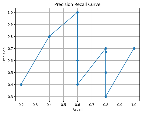
Using the trapezoidal rule, we calculate the area under the precision-recall curve, which yields an average precision of 0.84 after smoothing the curve. It’s important to note that this average precision value specifically pertains to one class (dog). This suggests that the model adeptly balances precision and recall, efficiently recognizing positive instances while mitigating false positives. This equilibrium signifies the model’s strong performance, offering a dependable trade-off between these crucial metrics.

Now that we’ve grasped the concept of Precision Average, let’s delve into Mean Average Precision (mAP)

Mean Average Precision(mAP)

Consider a scenario where you have a model that predicts if an image contains a dog, cat, bird, or fish. For each animal class, you evaluate the model’s performance by calculating precision and recall. This helps assess how effectively the model identifies instances of each animal.

After smoothing the curves, you find that the average precision for the dog class is 0.84, indicating that the model is good at correctly classifying dog images while minimizing false positives.

Now, let’s say you also calculate the average precision for the cat, bird, and fish classes, obtaining values of 0.78, 0.75, and 0.80 respectively. These values represent how well the model performs for each animal class individually.

To calculate the mean average precision (mAP), you simply average the average precision values obtained for each class. In this case:

mAP = (0.84 + 0.78 + 0.75 + 0.80) / 4 = 0.7925

So, the mean average precision for the model across all four classes is approximately 0.7925.

Conclusion

In conclusion, evaluation metrics are essential tools for evaluating and improving object detection methods. we’ve gained valuable insights and practical skills. We’ve learned how to measure the performance of object detection models using key metrics like IoU, precision, recall, mAP.

Through hands-on examples and Python code, we’ve mastered the art of calculating these metrics and interpreting their results. This newfound knowledge empowers us to assess model performance accurately and confidently.

.Moreover, by delving into visualizations like the Precision-Recall Curve we’ve gained a deeper understanding of model behavior and performance across different scenarios.

Overall, armed with this understanding and practical experience, we’re now better equipped to evaluate and improve object detection algorithms effectively. 

Have a question around this topic? Let us know in the comment section below or start a discussion at Analytics Vidhya Community!

Key Takeaways

• Learn why evaluation metrics matter in object detection, helping us assess how well detection methods perform in real  * world scenarios.
• We now know how to measure object detection performance using metrics like IoU, precision, recall, mAP.
• Gain insights into practical implementations of evaluation metrics through code examples and visualizations, making complex concepts easier to understand.We’ve learned to interpret visualizations like Precision-Recall Curve providing deeper insights into model behavior.
• Understand how evaluation metrics guide improvements in object detection models by identifying areas for refinement and optimization.
• Techniques like analyzing trade-offs and optimizing performance across thresholds help us evaluate and improve models effectively.

Frequently Asked Questions