Introduction
Decision trees, a fundamental tool in machine learning, are used for both classification and regression. With each internal node representing a decision based on a feature and each leaf node representing an outcome, decision trees mirror human decision-making processes, making them accessible and interpretable. Their versatility in handling both numerical and categorical data has made them indispensable across various domains such as finance, healthcare, and marketing. It acts as the base for more complex algorithms like Random Forest, XGBoost, and LightGBM.
Learning Objectives
- Gain a deep understanding of decision trees, including theoretical foundations such as standard deviation reduction, information gain, Gini impurity, and chi-square.
- Develop practical proficiency in implementing decision tree models using Python and scikit-learn, with step-by-step guidance and code explanations.
- Learn to use hyperparameter tuning for decision trees to optimize parameters such as maximum depth and minimum samples split, enhancing model performance and generalization capabilities.
Table of contents
- Introduction
- Anatomy of Decision Tree
- Different Decision Tree Algorithms
- What is Decision Node Splitting?
- What is Standard Deviation Reduction(SDR) ?
- What is Information Gain(IG)?
- What is Gini Index?
- What is Chi-square Test?
- What is Hyper parameter tuning?
- Step 1: Importing necessary libraries
- Step 2: Importing our dataset.
- Step 3: Now we will split the features and target variable
- Step 4: Using sklearn’s train_test_split method
- Step 5: Import the Decision Tree model from sklearn
- Step 6: Evaluation on our Decision Tree classifier
- Step 7: Finding Accuracy of Model
- Step 8: Implement Hyper Parameters of Decision Trees
- Step 9: Trying Hyper Parameter
- Step 10: Using the Hyper Parameter
- Step 12: Work with max_features
- Summary of Hyper parameter tuning
- Visualization of Decision Tree after Hyper Parameter Tuning
- Conclusion
- Frequently Asked Questions
Anatomy of Decision Tree
- Root Node: Top most node in the Decision Tree. Represents the entire dataset.
- Internal node: Nodes that are in the Decision Tree that are not lead nodes AKA Decision nodes.
- Leaf Node: Terminal node in Decision tree which represents the final outcome.
- Decision Rule: The path from root node to the lead node. Consists of a series of conditions.
- Splitting criterion: Criterion which is used to determine the partition of the dataset.
Different Decision Tree Algorithms
ID3(Iterative Dichotomiser 3): The algorithm constructs a multiway tree by iteratively selecting, in a greedy fashion, the categorical feature for each node that maximizes information gain with respect to categorical targets. Trees are expanded until their maximum size is reached, followed by a pruning step aimed at enhancing the tree’s capacity to generalize to new data.
C4.5: an advancement over ID3, eliminates the constraint of categorical features by dynamically defining discrete attributes based on numerical variables, partitioning continuous attribute values into intervals. It transforms the trained trees from the ID3 algorithm into sets of if-then rules. The accuracy of each rule is assessed to determine their sequence of application. Pruning involves removing a rule’s precondition if its accuracy improves without it.
C5.0: the latest version released by Quinlan, utilizes reduced memory and generates smaller rule sets compared to C4.5, all while achieving higher accuracy.
CART(Classification and Regression Trees): This shares similarities with C4.5, but diverges by accommodating numerical target variables for regression tasks and omitting the computation of rule sets. Instead, CART builds binary trees by selecting the feature and threshold combination that maximizes information gain at each node.
Sklearn uses an optimized version of CART, Sklearn implementation does not support categorical variables for now.
What is Decision Node Splitting?
A decision tree is built top-down from a root node and involves partitioning the data into subsets that contain instances with similar values (homogenous). We will be using Standard Deviation Reduction for continuous target variables and Gini, Information Gain and Chi-square for categorical target variables.
What is Standard Deviation Reduction(SDR) ?
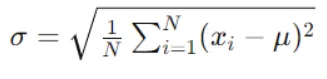
We use standard deviation to calculate the homogeneity of a numerical sample. If the numerical sample is completely homogeneous its standard deviation is zero.
Steps involved in Standard Deviation Reduction along with an example dataset:
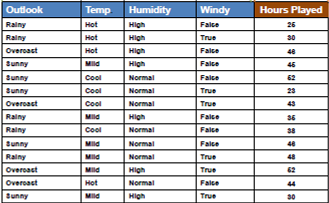
Step 1: Calculate the Standard Deviation (SD) for the Parent Node(Target Variable)
Compute the standard deviation of the target variable (or the variance, as both are proportional) for the data points in the current node. This represents the impurity or variability of the target variable within the node.
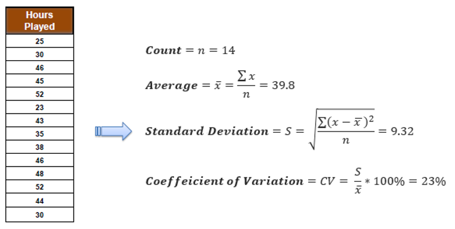
Step 2: Evaluate Standard Deviation for Each Feature
Determine the impact of splitting data on each feature on the standard deviation of the target variable. Compute the standard deviation for each child node resulting from the split and find the weighted average.
Similarly compute for other features as well.
Step 3: Compute Standard Deviation Reduction (SDR)
Subtract the weighted average of child node standard deviations from the parent node standard deviation. This value represents the reduction in standard deviation achieved by splitting on a feature.

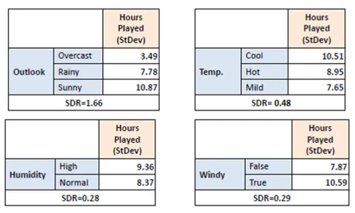
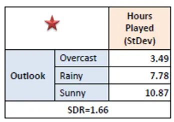
Step 4: Select Feature with Maximum SDR
Compare SDR values for all features. Choose the feature with the highest reduction in standard deviation as the splitting criterion.
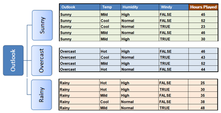
Step 5: Repeat Recursively
Split the dataset based on the selected feature into child nodes. Repeat the process recursively for each child node until stopping criteria are met.
In practice we need some termination criteria, we use coefficient of deviation(CV) and number of data points in our subset. Usually a threshold of 10% is set for CV and the minimum number of data points needed is 3.
After finding the feature for the decision node, if the feature is categorical then we split the decision node based on the classes present in that feature. If the feature is continuous then we follow the below steps to find the optimal split point.
Step 1: Sort the Feature Values: Arrange the feature in ascending order.
Step 2: Iterate through the features
For each unique feature value (excluding the last value):
Compute the reduction in SD by splitting the dataset into two groups:
- Group 1: Instances with feature values less than or equal to the current value.
- Group 2: Instances with feature values greater than the current value.
Calculate the SD for each group. Compute the weighted average of the SDs for both groups based on the number of instances in each group. Subtract the weighted average from the SD of the parent node to obtain the reduction in SD.
Step 3: Find the Optimal Split Point
Identify the split point that yields the maximum reduction in SD. This split point represents the optimal threshold for dividing the continuous feature into two subsets
Step 4: Split the Dataset
Split the dataset based on the chosen split point into two groups:
- Group 1: Instances with feature values less than or equal to the split point.
- Group 2: Instances with feature values greater than the split point.
Note: In sklearn library we can see that the criterion “squared error” has the implementation similar to Standard Deviation Reduction.
What is Information Gain(IG)?
IG quantifies the reduction in entropy (or uncertainty) achieved by splitting the data on a specific feature. Essentially, it measures how much more ordered the data becomes after the split compared to before. A higher information gain indicates that splitting the data on a particular feature results in more homogeneous subsets with respect to the target variable.
Steps involved in Information Gain along with an sample dataset:
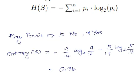
Step 1: Calculate Entropy for the Parent Node
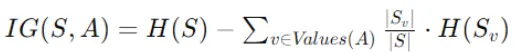
Compute the entropy of the target variable for the data points in the current node, representing uncertainty or impurity. Entropy measures the uncertainty or impurity of a dataset. For a given node S with n classes, entropy is calculated as:
Step 2: Evaluate Information Gain for Each Feature
Assess the reduction in entropy achieved by splitting the data on each feature. Compute the entropy for each child node resulting from the split and find the weighted average.
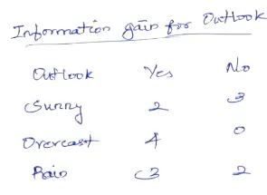
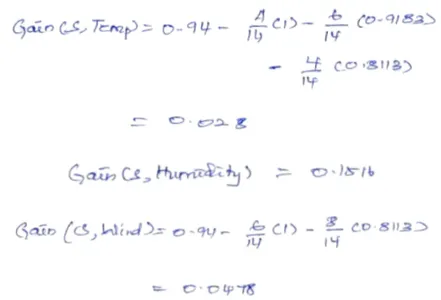
Information gain quantifies the reduction in entropy achieved by splitting the data on a particular feature. The formula for information gain is:
- IG(S,A) is the information gain for splitting node S using feature A.
- H(S) is the entropy of node S before the split.
- Values(A) represent the distinct values of feature A.
- ∣Sv∣ is the number of instances in node S with value v for feature A.
- ∣S∣ is the total number of instances in node S.
- H(Sv)is the entropy of the subset Sv of instances in node S with value v for feature A.
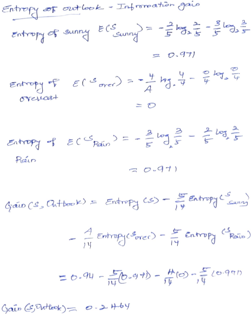
Similarly compute Information gain for other features as well.
Step 3: Compute Information Gain
Subtract the weighted average of child node entropies from the parent node entropy. This value represents the information gain obtained by splitting on a feature.
Step 4: Select Feature with Maximum Information Gain
Compare information gain values for all features. Choose the feature with the highest information gain as the splitting criterion.

Step 5: Repeat Recursively
Split the dataset based on the selected feature into child nodes. Repeat the process recursively for each child node until stopping criteria are met.
What is Gini Index?
The Gini index, also known as the Gini impurity, is a measure of impurity or inequality frequently used in decision tree algorithms, especially for classification tasks. It quantifies the likelihood of incorrectly classifying a randomly chosen element in a dataset.
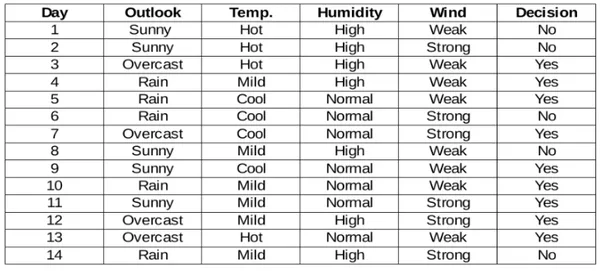
Steps involved in Gini Index with the example as Information gain:
Step 1: Calculate Gini Index for the Parent Node
Compute the Gini index of the target variable for the data points in the current node, representing impurity. Gini index is calculated as follows:
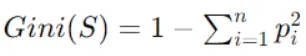
Where pi is the probability of class i in node S
Step 2: Evaluate Gini Index for Each Feature
Assess the reduction in Gini index achieved by splitting the data on each feature. Compute the Gini index for each child node resulting from the split.
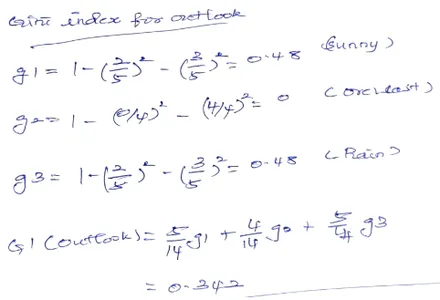
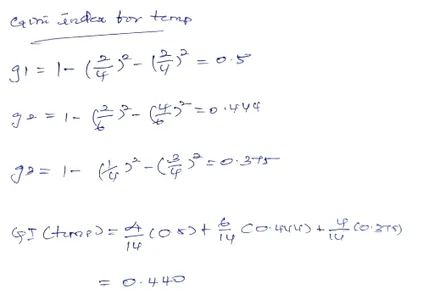

Step 3: Compute Gini Index Reduction
Subtract the weighted average of child node Gini indices from the Gini index of the parent node. This value represents the reduction in Gini index obtained by splitting on a feature.
Step 4: Select Feature with Maximum Gini Index Reduction
Compare Gini index reduction values for all features. Choose the feature with the highest reduction in Gini index as the splitting criterion.
Since we have GI of Outlook to be less we choose it as the root node.
Step 5: Repeat Recursively
Split the dataset based on the selected feature into child nodes. Repeat the process recursively for each child node until stopping criteria are met.
What is Chi-square Test?
Chi-square test is a statistical method used for feature selection. It assesses the independence between attributes (features) and the target variable. Specifically, the chi-square test evaluates whether there is a significant association between a categorical feature and the target variable in a dataset.
Steps involved in Chi-square Test:
Step 1: Calculate Contingency Table
Construct a contingency table (also known as a cross-tabulation table) that summarizes the frequency of occurrences for each combination of feature values and class labels.
Step 2: Compute Expected Frequencies
Calculate the expected frequencies for each cell in the contingency table under the assumption of independence between the feature and the target variable. This is done by multiplying the row and column totals and dividing by the grand total of observations.
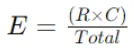
Expected Frequency (E) formula for a cell with row total (R) and column total (C) is:
Step 3: Calculate Chi-Square Statistic
Compute the Chi-Square statistic for each cell using the observed and expected frequencies. The formula for the Chi-Square statistic for a cell is:
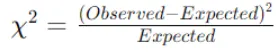
Sum the Chi-Square values across all cells to obtain the total Chi-Square statistic for the feature.
Step 4: Determine Degrees of Freedom
Determine the degrees of freedom (df) for the Chi-Square test, which is calculated as:
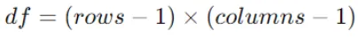
Where rows and columns are the number of categories in the feature and the target variable, respectively.
Now that we have seen the methods to split the Decision tree we will now look at the implementation of those.
For Detailed explanation of Chi Square, Please Refer CHAID.
What is Hyper parameter tuning?
Now let’s try some hyper parameter tuning on the decision tree. The goal from this hyper parameter tuning is to generalize the model and interpret decision trees at every point.
Step 1: Importing necessary libraries
import numpy as np
import pandas as pd
import matplotlib.pyplot as plt
import seaborn as sns
%matplotlib inline
Step 2: Importing our dataset.
We will be using Titanic dataset which is a preprocessed and encoded dataset.
data = pd.read_csv("data_cleaned.csv")
data.head()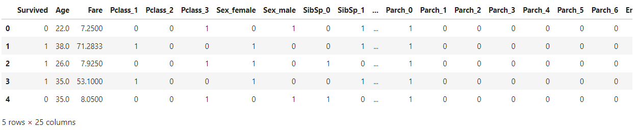
Step 3: Now we will split the features and target variable
X = data.drop(['Survived'], axis=1)
data['Survived'] = data['Survived'].astype(str)
y = data['Survived']
Step 4: Using sklearn’s train_test_split method
We will split the data into training and testing.
Deciding on the ratio depends on the dataset size, if you have a large dataset a smaller portion of the dataset can be allocated to test on the other hand with a smaller dataset you have to allocate enough data in the test for evaluation of the model’s performance. Here for simplicity we will use 75% train 25% test split.
from sklearn.model_selection import train_test_split
X_train, X_test, y_train, y_test = train_test_split(X, y,
test_size = 0.25, random_state = 42)
X_train.info()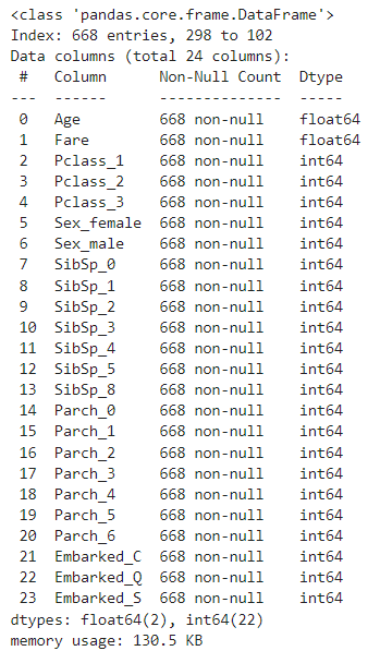
Step 5: Import the Decision Tree model from sklearn
We will import the Decision Tree model from sklearn. Then train our model with X_train and y_train. We will use random_state = 0 since the randomness of the estimator. The features are always randomly permuted at each split, even if splitter is set to “best”.
from sklearn.tree import DecisionTreeClassifier
clf = DecisionTreeClassifier(random_state=0)
clf.fit(X_train, y_train)
Step 6: Evaluation on our Decision Tree classifier
Now lets try some evaluation on our Decision Tree classifier, Below code will give us the confusion matrix.
from sklearn.metrics import confusion_matrix
confusion_matrix = confusion_matrix(y_test, y_pred_ti)
print("Confusion Matrix:\n", confusion_matrix)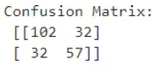
Step 7: Finding Accuracy of Model
We will find the training accuracy and testing accuracy of our model.
clf.score(X_train, y_train), clf.score(X_test, y_test)
We get our training accuracy to be around 98%. and our model got an accuracy of 71.3% which is very less compared to our training accuracy. Hence now we will be doing some hyper parameter tuning to our dataset in order to get a generalized model.
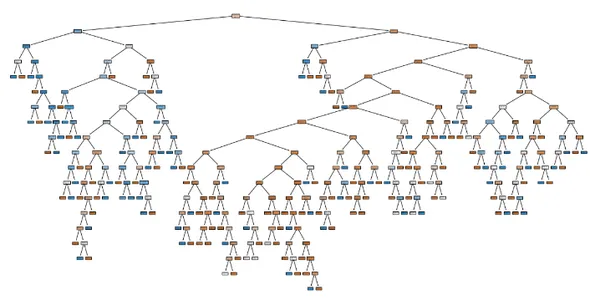
This is our decision tree before any hyper parameter tuning
from sklearn.tree import plot_tree
import matplotlib.pyplot as plt

# Visualize the decision tree
plt.figure(figsize=(20,10))  # Adjust the figure size as needed
plot_tree(clf, filled=True, feature_names=X_train.columns.tolist(),
class_names=clf.classes_.tolist())
plt.show()
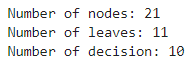
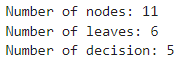
Code to know some information on DT:
import matplotlib.pyplot as plt
tree_info = clf.tree_
num_nodes = tree_info.node_count
num_leaves = tree_info.n_leaves
num_decision = num_nodes - num_leaves
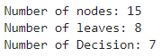
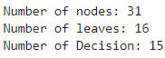
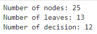
print("Number of nodes:", num_nodes)
print("Number of leaves:", num_leaves)
print("Number of decision:", num_decision)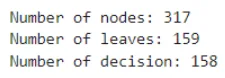
Step 8: Implement Hyper Parameters of Decision Trees
Let’s implement some hyper parameters of Decision Trees. Let’s try the max_depth parameter as this has the highest influence on our decision tree. max_depth allows the tree to grow deeper, as the tree grows deeper it captures intricate relationships in the data leading to better performance. However, it also increases the risk of overfitting, as the model memorizes the training data instead of generalizing.
We will start with max_depth = 3 and increase it accordingly. This acts like a regularization you impose constraints on the model’s complexity as the deeper decision tree gets more complex the model becomes.
clf = DecisionTreeClassifier(max_depth = 3, random_state=0)
clf.fit(X_train, y_train)
clf.score(X_train, y_train), clf.score(X_test, y_test)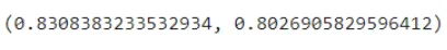
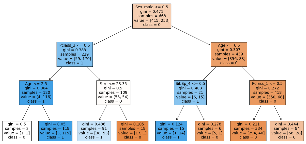
From our visualization we can see that 4 out of 8 of the leaf node contains proportions of our dataset. Hence we have to go deeper to capture more relationships. Hence we will increase the depth to 4.
We can see that the model is more generalized. Increasing depth more than 4 causes the model to overfit. After max_depth = 4 we can see that the model is overfitted.
Step 9: Trying Hyper Parameter
Now we will try out the other hyper parameter min_samples_split. As a thumb rule we can start with min_sample_split with 2 or 3 and increase until the model’s performance drops.
clf = DecisionTreeClassifier(max_depth = 4, min_samples_split = 15, random_state=0)
clf.fit(X_train, y_train)
clf.score(X_train, y_train), clf.score(X_test, y_test)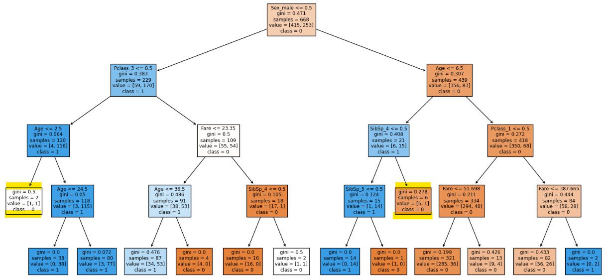
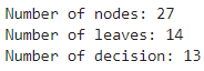
There is a reduction of two leaf nodes.
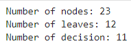
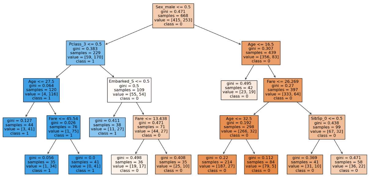
clf = DecisionTreeClassifier(max_depth = 4, min_samples_split = 16, random_state=0)
clf.fit(X_train, y_train)
clf.score(X_train, y_train), clf.score(X_test, y_test)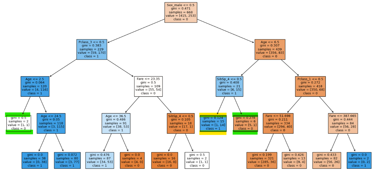
We can see that the highlighted node is not splitting because of our hyper parameter.
clf = DecisionTreeClassifier(max_depth = 4, min_samples_split = 19, random_state=0)
clf.fit(X_train, y_train)
clf.score(X_train, y_train), clf.score(X_test, y_te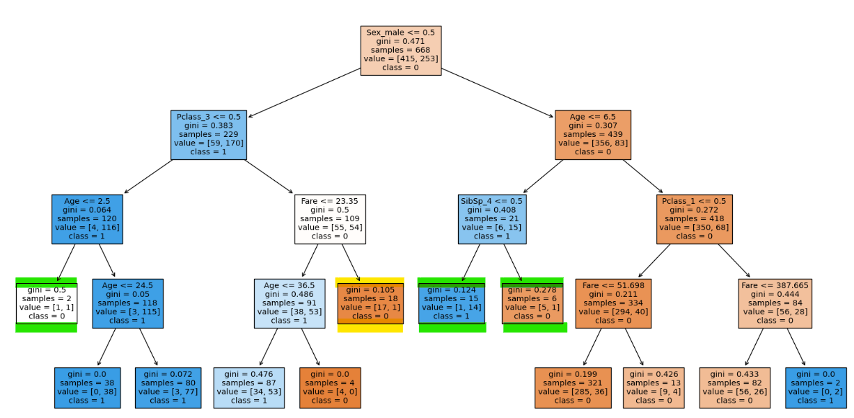
With min_samples_split 19 we can see that there is even more leaf nodes reduced with less compromise in testing accuracy.
Occam’s razor is a principle often attributed to. 14th–century friar William of Ockham says that if you have two competing ideas to explain the same phenomenon, you should prefer the simpler one.
We can see that with just a drop of 0.2% in accuracy we can get a simpler model hence we can go with the more generalized model than a complex one. Further increase in the min_samples_split generalizes the model causing it to underfit. Hence having min_samples_split 19 will make our model more simpler.
Step 10: Using the Hyper Parameter
Using the hyper parameter min_samples_leaf. A common guideline to the total number of samples in leaf nodes is set to 1% to 5%. Let’s go with the same and try some tuning.
Our dataset contains 668 data points hence 5% of it would be approx 35 we will try min_sample_leaf to be 35.
clf = DecisionTreeClassifier(max_depth = 4, min_samples_split = 19,
min_samples_leaf = 35, random_state=0)
clf.fit(X_train, y_train)
clf.score(X_train, y_train), clf.score(X_test, y_test)
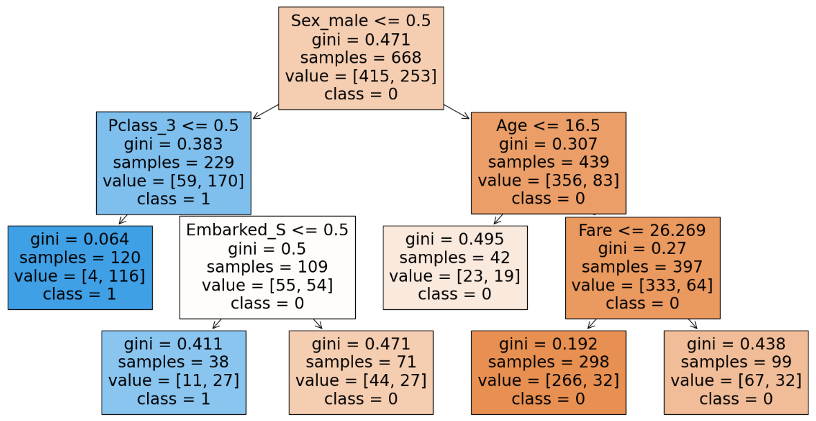
Here we can see that with the increase in the min_samples_leaf to 35 the training accuracy decreases but testing accuracy does not which means our model can handle unseen data even though the training accuracy is less. We can also see that the structure of the decision tree is different than before which has generalized. Hence we will stick with min_samples_leaf of 35. We can see that the number of nodes have decreased which means the model has been generalized.
Step 11: Working with max_leaf_nodes has shown us that with increase in the max_leaf_nodes until 6 has shown a positive impact where after 6 there was no change in the validation accuracy.
clf = DecisionTreeClassifier(max_depth = 4,  min_samples_split = 19,
min_samples_leaf = 35, max_leaf_nodes = 6, random_state=0)
clf.fit(X_train, y_train)
clf.score(X_train, y_train), clf.score(X_test, y_test)
We can infer that with occum’s razor that with a simpler model we get the same accuracy hence we will go with the simpler model and have max_leaf_nodes as 6.
Step 12: Work with max_features
Now lets work with max_features; default none.
clf = DecisionTreeClassifier(max_depth = 4, min_samples_split = 19,
min_samples_leaf = 35, max_leaf_nodes = 6, max_features = "log2", random_state=0)
clf.fit(X_train, y_train)
clf.score(X_train, y_train), clf.score(X_test, y_test)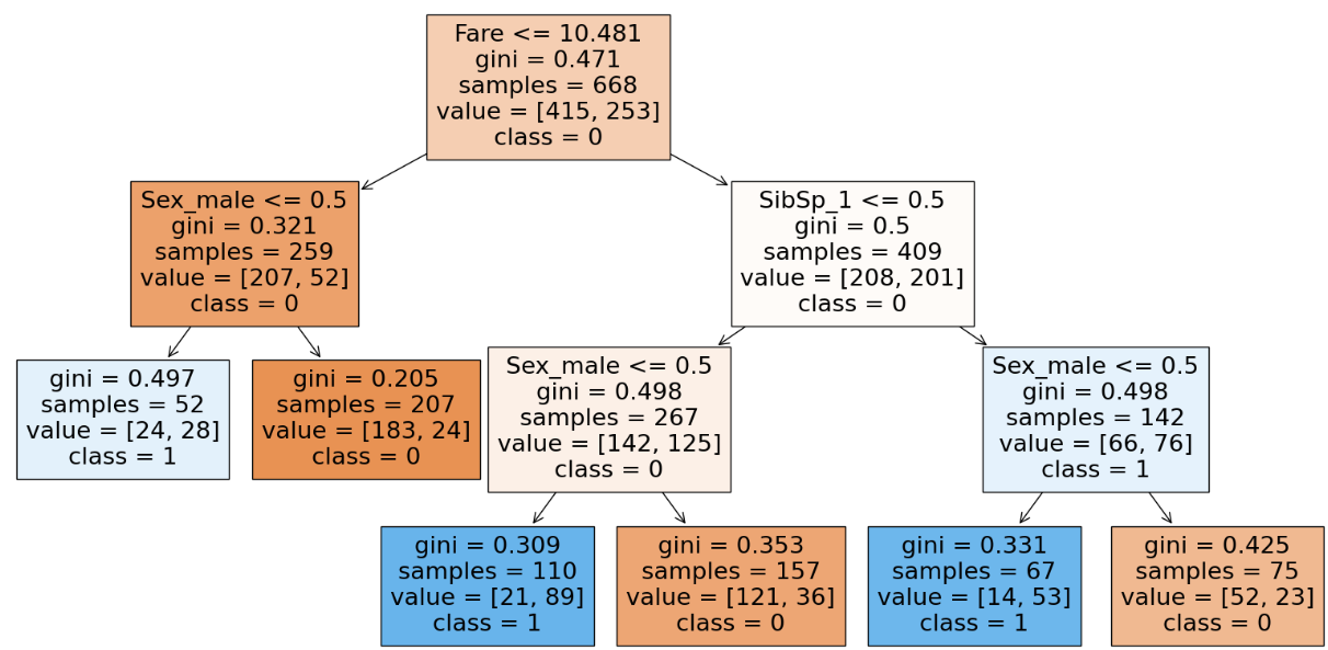
With the usage of max_feature we tend to decrease the training accuracy as we give less features to work with. This will happen only when we work with a dataset containing less features but when working with large datasets with hundreds of features using max_features will help as it reduces the computation to select the feature for the split. We can infer from the parameter(number of nodes) of the DT and realize that we are trying to generalize(decrease in accuracy) even more as the nodes decrease drastically. Hence there is a decrease in accuracy and chances of underfitting.
Summary of Hyper parameter tuning
| SL NO | Hyper parameter | Leaf Node and Decision Node | Training Accuracy | Testing Accuracy | Comments |
| 1 | Default | 159, 158 | 98.20 | 71.30 | Highly overfitted model. |
| 2 | max_depth = 3, rest default | 8, 7 | 83.08 | 80.2 | The model is generalized but there are chances of underfitting when max_depth reduced further. |
| 3 | max_depth = 4, rest default | 16, 15 | 84.28 | 80.71 | The model generalized and further increase in max_depth causes overfitting. |
| 4 | max_depth = 4, min_samples_split = 15, rest default | 14, 13 | 83.98 | 80.71 | More generalized model – since training and testing accuracy are getting closer. |
| 5 | max_depth = 4, min_samples_split = 16, rest default | 13, 12 | 83.98 | 80.71 | No change in accuracy with decrease in nodes means more generalization. |
| 6 | max_depth = 4, min_samples_split = 19, rest default | 12, 11 | 83.98 | 80.71 | More generalized than the previous one. |
| 7 | max_depth = 4, min_samples_split = 19, min_samples_leaf = 35, rest default | 11, 10 | 81.28 | 80.71 | More generalized than the previous one present in SL NO 3. Since the training and testing accuracies are even closer with less nodes. |
| 8 | max_depth = 4, min_samples_split = 19, min_samples_leaf = 35, max_leaf_nodes = 6, rest default | 6, 5 | 81.28 | 80.71 | With reference to accum’s razor concept we with two models having same accuracy, pick the model with less complexity. Here we can see that with 6 leaves and 5 decision nodes we are able to get the same accuracy as 11 leaves and 10 decision nodes hence we use max_leaf_nodes = 6. |
| 9 | max_depth = 4, min_samples_split = 19, min_samples_leaf = 35, max_leaf_nodes = 6,max_features = “log2”, rest default | 9, 8 | 78.74 | 78.47 | This could be an under fitted model since there is a decrease in both training and testing accuracies. Further tuning causes underfitting hence the previous model would be the best model. |
Visualization of Decision Tree after Hyper Parameter Tuning
from sklearn.tree import plot_tree
import matplotlib.pyplot as plt

plt.figure(figsize=(20,10))  # Adjust the figure size as needed
plot_tree(clf, filled=True, feature_names=X_train.columns.tolist(),
  class_names=clf.classes_.tolist())
plt.show()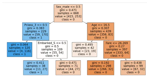
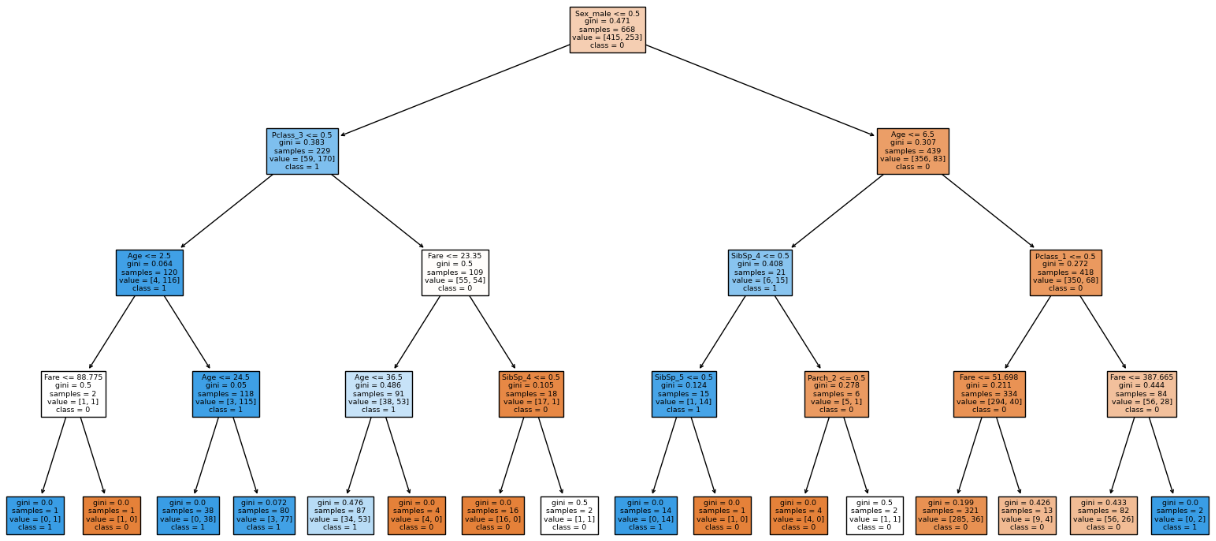
This will be the structure of the decision tree after hyper parameter tuning.
To know the hyper parameters of our decision tree:
params = clf.get_params()
print(params)
Conclusion
Decision trees represent a cornerstone in machine learning, offering a transparent and intuitive approach to solving classification and regression problems. Through methods like Information Gain, Gini Impurity, Standard Deviation Reduction, and Chi-Square, decision trees efficiently partition datasets, making them invaluable across diverse domains.
This article provided both theoretical insights and practical implementation guidance, enabling readers to construct decision tree models from scratch using Python and scikit-learn. By emphasizing the importance of hyperparameter tuning, readers gained proficiency in optimizing decision tree models for enhanced accuracy and generalization. Armed with this knowledge, practitioners are poised to leverage decision trees effectively in real-world applications, making informed decisions and driving impactful outcomes.
Frequently Asked Questions
Q1. What are the advantages of using decision trees over other machine learning models?
A. Decision trees offer transparency and interpretability, allowing users to understand the decision-making process easily. They can handle both numerical and categorical data, making them versatile across various domains. Additionally, decision trees can capture non-linear relationships in the data without the need for feature scaling.
Q2. How can I prevent overfitting in decision tree models?
A. Overfitting is a common concern in decision trees, especially with deep trees. To mitigate this, techniques such as pruning, setting a maximum tree depth, and using a minimum number of samples per leaf node can help control model complexity. Additionally, employing ensemble methods like Random Forests or Gradient Boosting can enhance generalization by aggregating multiple decision trees.
Q3. What are some common pitfalls to avoid when using decision trees?
A. One common pitfall is the tendency to create overly complex trees that memorize the training data (overfitting). It’s essential to strike a balance between model complexity and predictive performance. Another pitfall is the potential bias towards features with more categories or higher cardinality. Feature engineering and careful selection of splitting criteria can help address this issue. Lastly, decision trees may struggle with capturing interactions between features, especially in high-dimensional datasets. Feature engineering and ensemble methods can help mitigate this limitation.
Data science Trainee at Analytics Vidhya, specializing in ML, DL and Gen AI. Dedicated to sharing insights through articles on these subjects. Eager to learn and contribute to the field's advancements. Passionate about leveraging data to solve complex problems and drive innovation.


