Introduction

Decoding Neural Networks: Inspired by the intricate workings of the human brain, neural networks have emerged as a revolutionary force in the rapidly evolving domains of artificial intelligence and machine learning. However, before delving deeper into neural networks, it’s essential to grasp the distinction between machine learning and deep learning.

Within the realm of artificial intelligence, machine learning encompasses a broad spectrum of algorithms designed to learn from data and make predictions. Nonetheless, there’s a notable interest in deep learning, a subset of machine learning distinguished by its utilization of neural networks with multiple layers. This architectural complexity enables deep learning models to automatically glean intricate representations from data.

Deep learning finds preference in scenarios where conventional machine learning techniques may fall short. Applications dealing with complex patterns, vast datasets, and unstructured data find deep learning particularly suitable. Notably, deep learning excels in tasks such as image recognition, natural language processing, and audio analysis, owing to its innate ability to extract hierarchical features from raw data.

In many instances, deep learning surpasses traditional machine learning methods, especially in tasks requiring an in-depth comprehension of intricate data relationships. Its superiority becomes evident in situations where the scale and complexity of data necessitate a more sophisticated approach, rendering manual feature engineering impractical.

Learning Objective

• Understanding Neural Network
• Components of Neural Network
• Basic Components of Neural Network
• Optimizers in Neural Network
• Activation Functions in Neural Network

Understanding Neural Network

A neural network functions as a computational model inspired by the intricate neural networks present in the human brain. Similar to our brains, which consist of interconnected neurons, artificial neural networks consist of nodes or neurons organized into various layers. These layers collaborate to process information, enabling the neural network to learn and perform tasks.

In the realm of artificial intelligence, a neural network mimics the functionalities of the human brain. The overarching goal is to equip computers with the capability to reason and make decisions akin to humans. Achieving this objective involves programming computers to execute specific tasks, essentially simulating the interconnected nature of brain cells in a network. Essentially, a neural network acts as a potent tool within artificial intelligence, designed to replicate and utilize the problem-solving and decision-making prowess observed in the human brain.

Components of a Neural Network

Neurons

• Neurons are the fundamental units of a neural network, inspired by the neurons in the human brain.
• Each neuron processes information by receiving inputs, applying weights, and producing an output.
• Neurons in the input layer represents features, while those in the hidden layers perform computations and neurons in the output layer make final predictions.

Layers

• Neural networks are organized into layers, creating a hierarchical structure for information processing.
• Input Layer: It receives external information
• Hidden Layers: Perform complex computations, recognizing patterns and extracting features.
• Output Layers: Provides the final result or predictions.

Connections (Weights and Biases)

• Connections between neurons are represented by weights.
• Weights determine the strength of influence one neuron has on another.
• Biases are additional parameters that fine-tune the decision-making process.

Activation Functions

• Activation functions introduce non-linearity to the network, allowing it to capture complex patterns.
• Common activation functions include Sigmoid, Tanh, ReLU, Leaky ReLU, and SELU.

Basic Architecture of a Neural Network

Input Layer

• As the name suggests, the information in several different formats is provided, it is an entry point for external information into the neural network.
• Each neuron in this layer represents a specific feature of the input data.

Hidden Layers

• The hidden layer is present in between input and output layers
• It performs all the calculations to find hidden features and patterns.

Output Layer

• Input undergoes transformations in the hidden layer, leading to an output conveyed by this
  layer.
• The artificial neural network receives input and conducts a computation involving the weighted
  sum of input and a bias.
• This computation is represented in the form of a transfer function.

• Weighted sum is fed into an activation function to generate the output.
• Activation functions are pivotal in deciding if a node should activate, allowing only
  activated nodes to progress to the output layer.
• Various activation functions are available, and their selection depends on the specific
  task being performed.

Optimizing Input Layer Nodes in Neural Networks

Selecting the optimal number of nodes for the input layer in a neural network constitutes a critical decision influenced by the specific attributes of the dataset at hand.

A foundational principle involves aligning the quantity of input nodes with the features present in the dataset, with each node representing a distinct feature. This approach ensures thorough processing and capture of nuanced differences within the input data.

Furthermore, factors such as data dimensionality, including image pixel count or text vocabulary length, significantly impact the determination of input nodes.

Tailoring the input layer to task-specific requirements proves essential, particularly in structured data scenarios where nodes should mirror distinct dataset features or columns. Leveraging domain knowledge aids in identifying essential features while filtering out irrelevant or redundant ones, enhancing the network’s learning process. Through iterative experimentation and continual monitoring of the neural network’s performance on a validation set, the ideal number of input nodes undergoes iterative refinement.

Hidden layer learning in neural networks encompasses a sophisticated process during training, wherein hidden layers extract intricate features and patterns from input data.

Initially, neurons in the hidden layer receive meticulously weighted input signals, culminating in a transformation through an activation function. This non-linear activation enables the network to discern complex relationships within the data, empowering hidden layer neurons to specialize in recognizing specific features and capturing underlying patterns effectively.

The training phase further enhances this process through optimization algorithms like gradient descent, adjusting weights and biases to minimize discrepancies between predicted and actual outputs. This iterative feedback loop continues with backpropagation, refining hidden layers based on prediction errors. Overall, hidden layer learning is a dynamic process that transforms raw input data into abstract and representative forms, augmenting the network’s capacity for tasks such as classification or regression.

Determining Output Layer Neurons in Neural Networks

Deciding on the number of neurons in the output layer of a neural network is contingent upon the nature of the task being addressed. Here are key guidelines to aid in this decision-making process:

1. Classification Tasks:For classification tasks involving multiple classes, match the number of neurons in the output layer with the total classes.Utilize a softmax activation function to derive a probability distribution across the classes.
2. Binary Classification:In binary classification tasks with two classes (e.g., 0 or 1), employ a single neuron in the output layer.Implement a sigmoid activation function tailored for binary classification.
3. Regression Tasks:In regression tasks where the objective is to predict continuous values, opt for a single neuron in the output layer.Choose an appropriate activation function based on the range of the output (e.g., linear activation for unbounded outputs).
4. Multi-Output Tasks:For scenarios featuring multiple outputs, each representing distinct aspects of the prediction, adjust the number of neurons accordingly.Customize activation functions based on the characteristics of each output (e.g., softmax for categorical outputs, linear for continuous outputs).
5. Task-Specific Requirements:Align the number of neurons with the specific demands of the task at hand.Take into account the desired format of the network’s output and tailor the output layer accordingly to meet these requirements.

Activation Function

An activation function serves as a mathematical operation applied to each node in a neural network, particularly the output of a neuron within a neural network layer. Its primary role is to introduce non-linearities into the network, enabling it to recognize intricate patterns in the input data.

Once neurons in a neural network receive input signals and compute their weighted sum, they employ an activation function to generate an output. This function dictates whether a neuron should activate (fire) based on the weighted sum of its inputs.

List of Activation Functions

Sigmoid Function

• Formula:
• Range: (0,1)
• Sigmoid squashes the input values between 0 and 1, making it suitable for binary classification problems.

Hyperbolic Tangent Function(tanh)

• Formula: 
• Range: (-1,1)
• Similar to sigmoid, but with a range from -1 to 1. Tanh is often preferred in hidden layers, as it allows the model to capture both positive and negative relationships in the data.

Rectified Linear Unit (ReLu)

• Formula: ReLU(x) = max (0, x)
• Range: [0, ∞)
• ReLu is a popular choice due to its simplicity and efficiency. It sets negative values to zero and allows positive values to pass through, adding a level of sparsity to the network.

Leaky Rectified Linear Unit (Leaky ReLU)

• Formula: Leaky ReLU(x) = max (αx, x), where α is a small positive constant.
• Range:( -∞, ∞)
• Leaky ReLU address the “dying ReLU” problem by allowing a small positive gradient for negative inputs. It prevents neurons from becoming inactive during training.

Parametric Rectified Linear Unit (PReLU):

• Formula: PReLU(x)= max (αx, x), where α is a learnable parameter.
• Range: (-∞, ∞)
• Similar to Leaky ReLU but with the advantage of allowing the slope to be learned during training.

ELU

• Non-Linearity and Smoothness: It introduces non-linearity to the network, enabling it to learn complex relationships in data. ELU is smooth and differentiable everywhere, including at the origin, which can aid in optimization. –
• Mathematical Expression:

The ELU activation function is defined as: 

• Advantages
  • Handles Vanishing Gradients: ELU helps mitigate the vanishing gradient problem, which can be beneficial during the training of deep neural networks. 
  • Smoothness: The smoothness of the ELU function, along with its non-zero gradient for negative inputs, can contribute to more stable and robust learning.

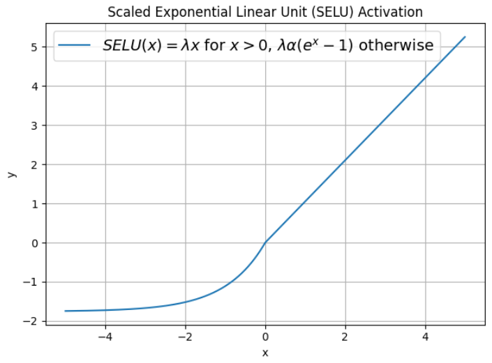
Scaled Exponential Linear Unit (SELU)

 Self-Normalizing Property

SELU possesses a self-normalizing property, which means that when used in deep neural networks,
it tends to maintain a stable mean and variance in each layer, addressing the vanishing and exploding gradient issues.

Mathematical Expression: The SELU activation function is defined as:

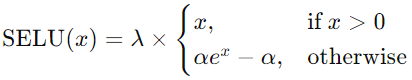
where α is the scale parameter and λ is the stability parameter

Advantages:

• Self-Normalization: The self-normalizing property of SELU aids in maintaining a stable distribution of activations during training, contributing to more effective learning in deep networks.
• Mitigates Vanishing/Exploding Gradients: SELU is designed to automatically scale the activations, helping to alleviate vanishing and exploding gradient problems.

Applicability: SELU is particularly useful in architectures with many layers, where maintaining stable gradients can be challenging.

Softmax Function

  Softmax is an activation function commonly used in the output layer of a neural network for multi-class classification tasks.

• Probability Distribution: It transforms the raw output scores into a probability distribution over multiple class.
• Mathematical Expression:

   The softmax function is defined as:

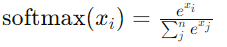
where xi​ is the raw score for class i, and max(x) is the maximum score across all classes.

• Properties:

• Normalization: Softmax ensures that the sum of probabilities for all classes equals 1, making it suitable for multi-class classification.
• Amplification of Differences: It amplifies the differences between the scores, emphasizing the prediction for the most probable class.

Use in Output Layer: Softmax is typically applied to the output layer of a neural network when the goal is to classify input into multiple classes. The class with the highest probability after softmax is often chosen as the predicted class.

Types of Neural Networks

Feedforward Neural Network (FNN)

• In this the input data type is Tabular data, fixed-size feature vectors.
• It is used for traditional machine learning tasks, such as binary or multi-class classification and regression.
• In this output layer activation for binary classification should be sigmoid, for multi-class classification Softmax and Linear Activation function.

Convolutional Neural Network (CNN)

• In this the Input Data Type is Grid-like data, such as images.
• It is used for image classification, object detection, image segmentation.
• In this the Output Layer Activation is Softmax for multi-class classification.

Recurrent Neural Network (RNN)

• In this the Input Data Type is Sequential data, such as time-series.
• It is used for Natural language processing, speech recognition, time-series prediction.
• In this the Output Layer Activation depends on the specific task; often Softmax for sequence classification.

Radial Basis Function Neural Network (RBFNN)

• Radial Basis Function Neural Network is a type of artificial neural network that is particularly suited for pattern recognition and spatial data analysis.
• It is used for Image recognition and medical diagnosis.
• In this output layer activation for binary classification should be sigmoid, for multi-class classification Softmax and Linear Activation function.

Autoencoder

• Autoencoders are particularly suitable for handling unlabelled data, often employed in dimensionality reduction.
• It is commonly used for feature learning, anomaly detection, and data compression.
• In this the output layer activation function is typically set to linear.

Guidelines for Selecting Neural Networks

• Choose FNN for traditional machine learning tasks with tabular data.
• Opt for CNN when dealing with grid-like data, especially images.
• Use RNN or LSTM for sequential data like time-series or natural language.
• Consider RBFNN for pattern recognition and spatial data.
• Apply Autoencoders for unsupervised learning, dimensionality reduction, and feature learning.

Neural Network Architectures: Understanding Input-Output Relationships

In neural networks, the relationship between input and output can vary, leading to distinct architectures based on the task at hand.

One-to-One Architecture

• In this architecture, a single input corresponds to a single output.
• Example: Predicting the sentiment of a text based on its content.
• Preferred Architecture: A standard feedforward neural network with hidden layers suffices for one-to-one tasks.

One-to-Many Architecture

• Here, a single input generates multiple outputs.
• Example: Generating multiple musical notes from a single input melody.
• Preferred Architecture: Sequence-to-Sequence models, such as Recurrent Neural Networks (RNNs) with attention mechanisms, are effective for one-to-many tasks.

Many-to-Many Architecture

• It involves multiple inputs mapped to multiple outputs.
• Example: Language translation, where a sentence in one language is translated into another.
• Preferred Architecture: Transformer models, leveraging attention mechanisms, are well-suited for many-to-many tasks.

Understanding the input-output relationships guides the selection of neural network architectures, ensuring optimal performance across diverse applications. Whether it’s a straightforward one-to-one task or a complex many-to-many scenario, choosing the right architecture enhances the network’s ability to capture intricate patterns in the data.

Loss Function

A loss function measures the difference between the predicted values of a model and the actual ground truth. The goal during training is to minimize this loss, aligning predictions with true values. The choice of the loss function depends on the task (e.g., MSE for regression, cross entropy for classification). It guides the model’s parameter adjustments, ensuring better performance. The loss function must be differentiable for gradient-based optimization. Regularization terms prevent overfitting, and additional metrics assess model performance. Overall, the loss function is crucial in training and evaluating machine learning models.

Regression in Loss Function in Neural Network

MSE (Mean Squared Error)

• It is the simplest and most common loss function.
• Measures the average squared difference between true and predicted values. Commonly used in regression tasks.
• When predicting the prices of houses, MSE is suitable. The squared nature of the loss heavily penalizes large errors, which is important for precise predictions in real estate.

MAE (Mean Absolute Error)

• It is the simplest and most common loss function.
• Calculates the average absolute difference between true and predicted values. Another common choice for regression problems.
• When estimating daily rainfall, MAE is appropriate. It gives equal weight to all errors and is less sensitive to outliers, making it suitable for scenarios where extreme values may occur.

Huber Loss

• Combines elements of MSE and MAE to be robust to outliers. Suitable for
  regression tasks.
• For predicting wind speed, where there might be occasional extreme values (outliers), Huber loss provides a balance between the robustness of MAE and the sensitivity of MSE.

• n – the number of data points.
• y – the actual value of the data point. Also known as true value.
• ŷ – the predicted value of the data point. This value is returned
  by the model.
• δ – defines the point where the Huber loss function transitions
  from a quadratic to linear.

Classification in Loss Function

Binary Cross-Entropy

• Used for binary classification problems, measuring the difference between true
  binary labels and predicted probabilities.
• When classifying emails as spam or not, binary cross-entropy is useful. It measures the difference between predicted probabilities and true binary labels, making it suitable for binary classification tasks.

• yi – actual values
• yihat – Neural Network prediction

Categorical Cross-Entropy

• Appropriate for multi-class classification, computing the loss between true
  categorical labels and predicted probabilities.  
• For image classification with multiple classes (e.g., identifying objects in images), categorical cross-entropy is appropriate. It considers the distribution of predicted probabilities across
  all classes.

These techniques are employed in various neural network architectures and tasks, depending on the nature of the problem and the desired characteristics of the model.

Backpropagation

Backpropagation is the process by which a neural network learns from its mistakes. It adjusts the weights of connections between neurons based on the errors made during the forward pass, ultimately refining its predictions over time.

This technique, known as backpropagation, is fundamental to neural network training. It entails propagating the error backwards through the layers of the network, allowing the system to fine-tune its weights.

Backpropagation plays a pivotal role in neural network training. By adjusting the weights based on the error rate or loss observed in previous iterations, it helps minimize errors and enhance the model’s generalizability and reliability.

With applications spanning various domains, backpropagation is a critical technique in neural network training, used for tasks such as:

• Image and Speech Recognition: Training neural networks to recognize patterns and features in images and speech.
• Natural Language Processing: Teaching models to understand and generate human language.
• Recommendation Systems: Building systems that provide personalized recommendations based on user behaviour.
• Regression and Classification: In tasks where the goal is to predict continuous values (regression) or classify inputs into categories(classification)A key component of deep neural network training is backpropagation, which allows weights to be adjusted iteratively, allowing the network to learn and adapt to complicated patterns in the input. 

Optimizers

Stochastic Gradient Descent (SGD)

• SGD is a fundamental optimization algorithm that updates the model’s parameters using the gradients of the loss with respect to those parameters. It performs a parameter update for each training example, making it computationally efficient but more prone to noise in the updates.
• It is Suitable for large datasets and simple models.

RMSprop (Root Mean Square Propagation)

• RMSprop adapts the learning rates of each parameter individually by dividing the learning rate for a weight by a running average of the magnitudes of recent gradients for that weight. It helps handle uneven gradients and accelerate convergence.
• It is Effective for non-stationary environments or problems with sparse data.

Adam (Adaptive Moment Estimation)

• Adam combines the ideas of momentum and RMSprop. It maintains moving averages of both the gradients and the second moments of the gradients. It adapts the learning rates for each parameter individually and includes bias correction terms.
• It is widely used in various applications due to its robust performance across different types of datasets.

AdamW

• AdamW is a modification of Adam that incorporates weight decay directly into the optimization process. It helps prevent overfitting by penalizing large weights.
• It is useful for preventing overfitting, particularly in deep learning models.

Adadelta

• Adadelta is an extension of RMSprop that eliminates the need for manually setting a learning rate. It uses a running average of squared parameter updates to adaptively adjust the learning rates during training.
• It is suitable for problems with sparse gradients and when manual tuning of learning rates is challenging.

These optimizers are crucial for training neural networks efficiently by adjusting the model parameters during the learning process. The choice of optimizer depends on the specific characteristics of the dataset and the problem at hand.

Building your First Neural Network

Let’s create a simple neural network for a very basic dataset. We’ll use the sklearn.datasets ‘make_classification’ function to generate a synthetic binary classification dataset:

First make sure to run these commands in your terminal or command prompt before running the provided code.

pip install numpy matplotlib scikit-learn tensorflow

Importing Required Libraries

import numpy as np

import matplotlib.pyplot as plt

from sklearn.datasets import make_classification

from sklearn.model_selection import train_test_split

import tensorflow as tf

from tensorflow.keras import layers, models

Generating a Synthetic binary classification dataset

X, y = make_classification(n_samples=1000, n_features=2, n_classes=2, n_clusters_per_class=1, n_redundant=0, random_state=42)

Split the data into traing and testing sets

X_train, X_test, y_train, y_test = train_test_split(X, y, test_size=0.2, random_state=42)

Define the model

model = models.Sequential()

model.add(layers.Dense(units=1, activation='sigmoid', input_shape=(2,)))

Compile the model

model.compile(optimizer='adam', loss='binary_crossentropy', metrics=['accuracy'])

Train the model

history = model.fit(X_train, y_train, epochs=20, batch_size=32, validation_split=0.2)

Evaluate the model on the test set

test_loss, test_accuracy = model.evaluate(X_test, y_test)

print(f'Test Accuracy: {test_accuracy * 100:.2f}%')

In this example, we generate a simple synthetic binary classification dataset with two features. The neural network has one output unit with a sigmoid activation function for binary classification.

This is a basic example to help you get started with building and training a neural network on a simple dataset.

Conclusion

This article explores neural networks’ transformative impact on AI and machine learning, drawing inspiration from the human brain. Deep learning, a subset of machine learning, employs multi-layered neural networks for complex learning. The diverse network types, adaptable to tasks like image recognition and natural language processing, highlight their versatility. Activation functions introduce crucial non-linearity, capturing intricate patterns. Careful selection of functions and architectures is pivotal. A comprehensive grasp of neural networks enables effective utilization of deep learning’s potential across diverse domains, promising ongoing innovation in AI and ML.

Want to upgrade your skills and become a data scientist? Enroll today for our AI and ML Blackbelt Plus program!

Frequently Asked Questions