Introduction
Last week, I wrote an introductory article on the package data.table. It was intended to provide you a head start and become familiar with its unique and short syntax. The next obvious step is to focus on modeling, which we will do in this post today.
With data.table, you no longer need to worry about your machine cores’ (or RAM to some extent). Atleast, I used to think of myself as a crippled R user when faced with large data sets. But not anymore! I would like to thank Matt Dowle again for this accomplishment.
Last week, I received an email saying:
Okay, I get it. data.table empowers us to do data exploration & manipulation. But, what about model building ? I work with 8GB RAM. Algorithms like random forest (ntrees = 1000) takes forever to run on my data set with 800,000 rows.
I’m sure there are many R users who are trapped in a similar situation. To overcome this painstaking hurdle, I decided to write this post which demonstrates using the two most powerful packages i.e. H2O and data.table.
For practical understanding, I’ve taken the data set from a practice problem and tried to improve the score using 4 different machine learning algorithms (with H2O) & feature engineering (with data.table). So, get ready for a journey from rank 154th to 25th on the leaderboard.

Table of Contents
- What is H2o ?
- What makes it faster ?
- Solving a Problem
- Getting Started
- Data Exploration using data.table and ggplot
- Data Manipulation using data.table
- Model Building (using H2O)
- Regression
- Random Forest
- GBM
- Deep Learning
Note: Consider this article as a starters guide for model building using data.table and H2O. I haven’t explained these algorithms in details. Rather, the focus is kept on implementing these algorithms using H2O. Dont worry, links to resources are provided.
What is H2O ?
 H2O is an open source machine learning platform where companies can build models on large data sets (no sampling needed) and achieve accurate predictions. It is incredibly fast, scalable and easy to implement at any level.
In simple words, they provide a GUI driven platform to companies for doing faster data computations. Currently, their platform supports advanced & basic level algorithms such as deep learning, boosting, bagging, naive bayes, principal component analysis, time series, k-means, generalized linear models.
In addition, H2O has released APIs for R, Python, Spark, Hadoop users so that people like us can use it to build models at individual level. Needless to say, it’s free to use and instigates faster computation.
What makes it faster ?
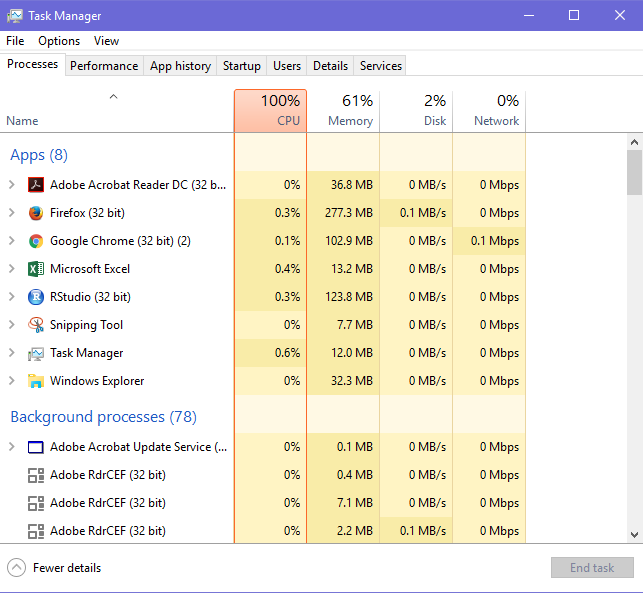
H2O has a clean and clear feature of directly connecting the tool (R or Python) with your machine’s CPU. This way we get to channelize more memory, processing power to the tool for making faster computations. This will allow computations to take place at 100% CPU capacity (shown below). It can also be connected with clusters at cloud platforms for doing computations.
Along with, it uses in-memory compression to handle large data sets even with a small cluster. It also include provisions to implement parallel distributed network training.
Tip: In order to channelize all your CPU’s processing power for model computation, avoid using any application or software which consumes too much memory. Specially, avoid opening too many tabs on google chrome or any other web browser.
Solving a Problem
Let’s get down to use these package and build some nice models.
1. Getting Started
Data Set: I’ve taken the data set from Black Friday Practice Problem. The data set has two parts: Train and Test. Train data set contains 550068 observations. Test data set contains 233599 observations. To download the data and read the problem statement: Click Here. One time login will be required.
Let’s get started!
Ideally, the first step in model building is hypothesis generation. This step is carried out after you have read the problem statement but not seen the data.
Since, this guide isn’t designed to demonstrate all predictive modeling steps, I leave that upto you. Here’s a good resource to freshen up your basics: Guide to Hypothesis Generation. If you do this step, may be you could end up creating a better model than mine. Do give your best shot.
Starting with loading data in R.
> path <- "C:/Users/manish/desktop/Data/H2O"
> setwd(path)
#install and load the package
> install.packages("data.table")
> library(data.table)
#load data using fread
> train <- fread("train.csv", stringsAsFactors = T)
> test <- fread("test.csv", stringsAsFactors = T)
Within seconds, fread loads the data in R. It’s that fast. The parameter stringsAsFactors ensures that character vectors are converted into factors. Let’s quickly check the data set now.
#No. of rows and columns in Train
> dim(train)
[1] 550068 12
#No. of rows and columns in Test
> dim(test)
[1] 233599 11
> str(train)
Classes ‘data.table’ and 'data.frame': 550068 obs. of 12 variables:
$ User_ID : int 1000001 1000001 1000001 1000001 1000002 1000003 1000004 1000004 1000004...
$ Product_ID : Factor w/ 3631 levels "P00000142","P00000242",..: 673 2377 853 829 2735 2632
$ Gender : Factor w/ 2 levels "F","M": 1 1 1 1 2 2 2 2 2 2 ...
$ Age : Factor w/ 7 levels "0-17","18-25",..: 1 1 1 1 7 3 5 5 5 3 ...
$ Occupation : int 10 10 10 10 16 15 7 7 7 20 ...
$ City_Category : Factor w/ 3 levels "A","B","C": 1 1 1 1 3 1 2 2 2 1 ...
$ Stay_In_Current_City_Years: Factor w/ 5 levels "0","1","2","3",..: 3 3 3 3 5 4 3 3 3 2 ...
$ Marital_Status : int 0 0 0 0 0 0 1 1 1 1 ...
$ Product_Category_1 : int 3 1 12 12 8 1 1 1 1 8 ...
$ Product_Category_2 : int NA 6 NA 14 NA 2 8 15 16 NA ...
$ Product_Category_3 : int NA 14 NA NA NA NA 17 NA NA NA ...
$ Purchase : int 8370 15200 1422 1057 7969 15227 19215 15854 15686 7871 ...
- attr(*, ".internal.selfref")=<externalptr>
What do we see ? I see 12 variables, 2 of which seems to have so many NAs. If you have read the problem description and data information, we see Purchase is the dependent variable, rest 11 are independent variables.
Looking at the nature of Purchase variable (continuous), we can infer that this is a regression problem. Even though, the competition is closed but we can still check our score and evaluate how good we could have done. Let’s make our first submission.
With all the data points we’ve got, we can make our first set of prediction using mean. This is because, mean prediction will give us a good approximation of prediction error. Taking this as baseline prediction, our model won’t do worse than this.
#first prediction using mean
> sub_mean <- data.frame(User_ID = test$User_ID, Product_ID = test$Product_ID, Purchase = mean(train$Purchase))
> write.csv(sub_mean, file = "first_sub.csv", row.names = F)
It was this simple. Now, I’ll upload the resultant file and check my score and rank. Don’t forget to convert .csv to .zip format before you upload. You can upload and check your solution at the competition page.
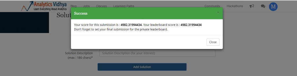
Our mean prediction gives us a mean squared error of 4982.3199. But, how good is it? Let’s check my ranking on leaderboard.
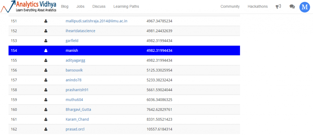
Thankfully, I am not last. So, mean prediction got me 154 / 162 rank. Let’s improve this score and attempt to rise up the leader board.
Before starting with univariate analysis, let’s quick summarize both the files (train and test) and decipher, if there exist any disparity.
> summary (train)
> summary (test)
Look carefully (check at your end) , do you see any difference in their outputs? Actually, I found one. If you carefully compare Product_Category_1, Product_Category_2 & Product_Category_3 in test and train data, there exist a disparity in max value. max value of Product_Category_1 is 20 whereas for others is 18. These extra category levels appears to be noise. Make a note this this. We’ll need to remove them.
Let’s combine the data set. I’ve used rbindlist function from data.table, since it’s faster than rbind.
#combine data set
> test[,Purchase := mean(train$Purchase)]
> c <- list(train, test)
> combin <- rbindlist(c)
In the code above, we’ve first added the Purchase variable in the test set so that both data sets have equal number of columns. Now, we’ll do some data exploration.
2. Data Exploration using data.table & ggplot
In this section, we’ll do some univariate and bivariate analysis, and try to understand the relationship among given variables. Let’s start with univariate.
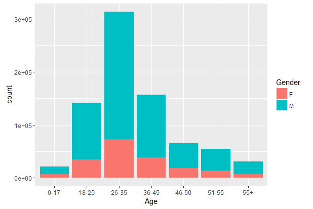
#analyzing gender variable
> combin[,prop.table(table(Gender))]
Gender

F          M

0.2470896 0.7529104
#Age Variable
> combin[,prop.table(table(Age))]
Age
0-17 18-25 26-35 36-45 46-50 51-55 55+
0.02722330 0.18113944 0.39942348 0.19998801 0.08329814 0.06990724 0.03902040
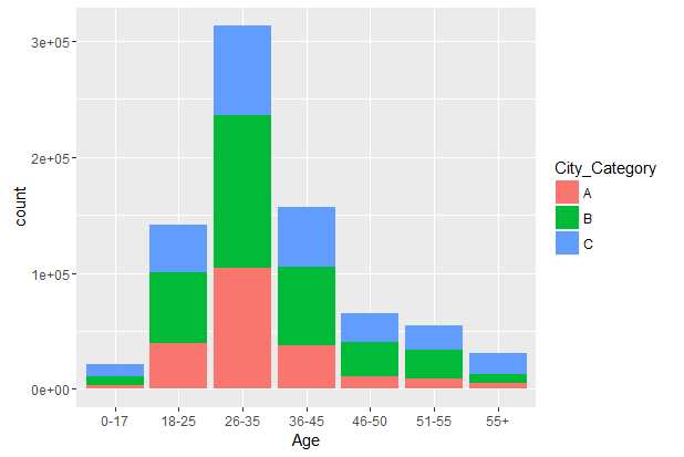
#City Category Variable
> combin[,prop.table(table(City_Category))]
City_Category
A B C
0.2682823 0.4207642 0.3109535
#Stay in Current Years Variable
> combin[,prop.table(table(Stay_In_Current_City_Years))]
Stay_In_Current_City_Years
0 1 2 3 4+
0.1348991 0.3527327 0.1855724 0.1728132 0.1539825
#unique values in ID variables
> length(unique(combin$Product_ID))
[1] 3677
>length(unique(combin$User_ID))
[1] 5891
#missing values
> colSums(is.na(combin))
User_ID Product_ID
0 0
Gender Age
0 0
Occupation City_Category
0 0
Stay_In_Current_City_Years Marital_Status
0 0
Product_Category_1 Product_Category_2
0 245982
Product_Category_3 Purchase
545809 0
Following are the inferences we can generate from univariate analysis:
- We need to encode Gender variable into 0 and 1 (good practice).
- We’ll also need to re-code the Age bins.
- Since there are three levels in City_Category, we can do one-hot encoding.
- The “4+” level of Stay_in_Current_Years needs to be revalued.
- The data set does not contain all unique IDs. This gives us enough hint for feature engineering.
- Only 2 variables have missing values. In fact, a lot of missing values, which could be capturing a hidden trend. We’ll need to treat them differently.
We’ve got enough hints from univariate analysis. Let’s tap out bivariate analysis quickly. You can always make these graphs look beautiful by adding more parameters. Here’s a quick guide to learn making ggplots.
> library(ggplot2)
#Age vs Gender
> ggplot(combin, aes(Age, fill = Gender)) + geom_bar()
#Age vs City_Category
ggplot(combin, aes(Age, fill = City_Category)) + geom_bar()
We can also create cross tables for analyzing categorical variables. To make cross tables, we’ll use the package gmodels which creates comprehensive cross tables.
> library(gmodels)
> CrossTable(combin$Occupation, combin$City_Category)
With this, you’ll obtain a long comprehensive cross table of these two variables. Similarly, you can analyze other variables at your end. Our bivariate analysis haven’t provided us much actionable insights. Anyways, we get to data manipulation now.
3. Data Manipulation using data.table
In this part, we’ll create new variables, revalue existing variable and treat missing values. In simple words, we’ll get our data ready for modeling stage.
Let’s start with missing values. We saw Product_Category_2 and Product_Category_3 had a lot of missing values. To me, this suggests a hidden trend which can be mapped by creating a new variable. So, we’ll create a new variable which will capture NAs as 1 and non-NAs as 0 in the variables Product_Category_2 and Product_Category_3.
#create a new variable for missing values
> combin[,Product_Category_2_NA := ifelse(sapply(combin$Product_Category_2, is.na) == TRUE,1,0)]
> combin[,Product_Category_3_NA := ifelse(sapply(combin$Product_Category_3, is.na) == TRUE,1,0)]
Let’s now impute the missing values with any arbitrary number. Let’s take -999
#impute missing values
> combin[,Product_Category_2 := ifelse(is.na(Product_Category_2) == TRUE, "-999", Product_Category_2)]
> combin[,Product_Category_3 := ifelse(is.na(Product_Category_3) == TRUE, "-999", Product_Category_3)]
Before proceeding to feature engineering, lastly, we’ll revalue variable levels as inferred from our univariate analysis.
#set column level
> levels(combin$Stay_In_Current_City_Years)[levels(combin$Stay_In_Current_City_Years) == "4+"] <- "4"
#recoding age groups
> levels(combin$Age)[levels(combin$Age) == "0-17"] <- 0
> levels(combin$Age)[levels(combin$Age) == "18-25"] <- 1
> levels(combin$Age)[levels(combin$Age) == "26-35"] <- 2
> levels(combin$Age)[levels(combin$Age) == "36-45"] <- 3
> levels(combin$Age)[levels(combin$Age) == "46-50"] <- 4
> levels(combin$Age)[levels(combin$Age) == "51-55"] <- 5
> levels(combin$Age)[levels(combin$Age) == "55+"] <- 6
#convert age to numeric
> combin$Age <- as.numeric(combin$Age)
#convert Gender into numeric
> combin[, Gender := as.numeric(as.factor(Gender)) - 1]
It is advisable to convert factor variables into numeric or integer for modeling purpose.
Let’s now move one step ahead, and create more new variables a.k.a feature engineering. To know more about feature engineering, you can read more.
During univariate analysis, we discovered that ID variables have lesser unique values as compared to total observations in the data set. It means there are User_IDs or Product_IDs must have appeared repeatedly in this data set.
Let’s create a new variable which captures the count of these ID variables. Higher user count suggests that a particular user has purchased products multiple times. High product count suggests that a product has been purchased many a times, which shows its popularity.
#User Count
> combin[, User_Count := .N, by = User_ID]
#Product Count
> combin[, Product_Count := .N, by = Product_ID]
Also, we can calculate the mean purchase price of a product. Because, lower the purchase price, higher will be the chances of that product being bought or vice versa. Similarly, we can create another variable which maps the average purchase price by user i.e. how much purchase (on an average) is made by a user. Let’s do it.
#Mean Purchase of Product
> combin[, Mean_Purchase_Product := mean(Purchase), by = Product_ID]
#Mean Purchase of User
> combin[, Mean_Purchase_User := mean(Purchase), by = User_ID]
Now, we are only left with one hot encoding of City_Category variable. This can be done in one line using library dummies.
> library(dummies)
> combin <- dummy.data.frame(combin, names = c("City_Category"), sep = "_")
Before, proceeding to modeling stage, let’s check data types of variables once, and make the required changes, if necessary.
#check classes of all variables
> sapply(combin, class)
#converting Product Category 2 & 3
> combin$Product_Category_2 <- as.integer(combin$Product_Category_2)
> combin$Product_Category_3 <- as.integer(combin$Product_Category_3)
4. Model Building using H2O
In this section, we’ll explore the power of different machine learning algorithms in H2O. We’ll build models with Regression, Random Forest, GBM and Deep Learning.
Make sure you don’t use these algorithms like a black box. It is advisable to know how do they work. This will help you to understand the parameters used in building these models. Here are some useful resources to learn about these algorithms:
- Regression: Starters Guide to Regression
- Random Forest, GBM: Starters Guide to Tree Based Algorithms
- Deep Learning: Starters Guide to Deep Learning
But, first things first. Let’s divide the data set into test and train.
#Divide into train and test
> c.train <- combin[1:nrow(train),]
> c.test <- combin[-(1:nrow(train)),]
As discovered in beginning that the variable Product_Category_1 in train has some noise. Let’s remove it as well by selecting all rows in Product_Category_1 upto 18, thereby dropping rows which has category level 19 & 20.
> c.train <- c.train[c.train$Product_Category_1 <= 18,]
Now, our data set is ready for modeling. Time to install H2O package in R. The procedure to load package remains same. For faster computation make sure, you’ve closed all other applications. So, how does H2O in R work ? It’s simple actually!
R uses REST API as a reference object to send functions, data to H2O. The data set is then assigned a key for future reference. H2O doesn’t uses .csv data, instead it converts .csv to its own H2O instance data. You’d be surprised to know that H2O has its own functions for data manipulation too. But, data.table is no bad either.
> install.packages("h2o")
> library(h2o)
To launch the H2O cluster, write –
> localH2O <- h2o.init(nthreads = -1)
This commands tell H2O to use all the CPUs on the machine, which is recommended. For larger data sets (say > 1,000,000 rows), h2o recommends running cluster on a server with high memory for optimal performance. Once the instance starts successfully, you can also check its status using:
> h2o.init()
Connection successful!
R is connected to the H2O cluster:
H2O cluster uptime: 1 days 9 hours
H2O cluster version: 3.8.1.3
H2O cluster name: H2O_started_from_R_manish_vkt788
H2O cluster total nodes: 1
H2O cluster total memory: 1.50 GB
H2O cluster total cores: 4
H2O cluster allowed cores: 4
H2O cluster healthy: TRUE
H2O Connection ip: localhost
H2O Connection port: 54321
H2O Connection proxy: NA
R Version: R version 3.2.2 (2015-08-14)
Let’s now transfer the data from R to h2o instance. It can be accomplished using as.h2o command.
#data to h2o cluster
> train.h2o <- as.h2o(c.train)
> test.h2o <- as.h2o(c.test)
Using column index, we need to identify variables to be used in modeling as follows:
#check column index number
> colnames(train.h2o)
[1] "User_ID" "Product_ID"
[3] "Gender" "Age"
[5] "Occupation" "City_Category_A"
[7] "City_Category_B" "City_Category_C"
[9] "Stay_In_Current_City_Years" "Marital_Status"
[11] "Product_Category_1" "Product_Category_2"
[13] "Product_Category_3" "Purchase"
[15] "Product_Category_2_NA" "Product_Category_3_NA"
[17] "User_Count" "Product_Count"
[19] "Mean_Purchase_Product" "Mean_Purchase_User"
#dependent variable (Purchase)
> y.dep <- 14
#independent variables (dropping ID variables)
> x.indep <- c(3:13,15:20)
Let’s start with Multiple Regression model.
Multiple Regression in H2O
> regression.model <- h2o.glm( y = y.dep, x = x.indep, training_frame = train.h2o, family = "gaussian")
> h2o.performance(regression.model)
H2ORegressionMetrics: glm
** Reported on training data. **
MSE: 16710563
R2 : 0.3261543
Mean Residual Deviance : 16710563
Null Deviance :1.353804e+13
Null D.o.F. :545914
Residual Deviance :9.122547e+12
Residual D.o.F. :545898
AIC :10628689
GLM algorithm in H2O can be used for all types of regression such as lasso, ridge, logistic, linear etc. A user only needs to modify the family parameter accordingly. For example: To do logistic regression, you can write family = “binomial”.
So, after we print the model results, we see that regression gives a poor R² value i.e. 0.326. It means that only 32.6% of the variance in the dependent variable is explained by independent variable and rest is unexplained. This shows that regression model is unable to capture non linear relationships.
Out of curiosity, let’s check the predictions of this model. Will it be worse than mean predictions ? Let’ see.
#make predictions
> predict.reg <- as.data.frame(h2o.predict(regression.model, test.h2o))
> sub_reg <- data.frame(User_ID = test$User_ID, Product_ID = test$Product_ID, Purchase = predict.reg$predict)
> write.csv(sub_reg, file = "sub_reg.csv", row.names = F)
Let’s upload the solution file (in .zip format) and check if we have got some improvement.

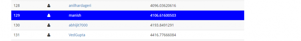
Wow! Our prediction score has improved. We started from 4982.31 and with regression we’ve got an improvement over previous score. On leaderboard, this submission takes me to 129th position.
It seems, we can do well if we choose an algorithm which maps non-linear relationships well. Random Forest is our next bet. Let’s do it.
Random Forest in H2O
#Random Forest
> system.time(
rforest.model <- h2o.randomForest(y=y.dep, x=x.indep, training_frame = train.h2o, ntrees = 1000, mtries = 3, max_depth = 4, seed = 1122)
)
# |====================================================================| 100%
# user system elapsed
# 21.85 1.61 2260.33
With 1000 trees, random forest model took approx ~38 minutes to run. It operated at 100% CPU capacity which can be seen in Task Manager (shown below).
Your model might not take same time because of difference in our machine specifications. Also, I had to open web browsers which consumed a lot of memory. Actually, your model might take lesser time. You can check the performance of this model using the same command as used previously:
> h2o.performance(rforest.model)
#check variable importance
> h2o.varimp(rforest.model)
Let’s check the leaderboard performance of this model by making predictions. Do you think our score will improve ? I’m a little hopeful, though!
#making predictions on unseen data

> system.time(predict.rforest <- as.data.frame(h2o.predict(rforest.model, test.h2o)))
# |====================================================================| 100%
# user system elapsed
# 0.44 0.08 21.68
#writing submission file
> sub_rf <- data.frame(User_ID = test$User_ID, Product_ID = test$Product_ID, Purchase = predict.rforest$predict)
> write.csv(sub_rf, file = "sub_rf.csv", row.names = F)
Making predictions took ~ 22 seconds. Now is the time to upload the submission file and check the results.

Random Forest was able to map non-linear relations way better than regression ( as expected). With this score, my ranking on leaderboard moves to 122:

This gave a slight improvement on leaderboard, but not as significant as expected. May be GBM, a boosting algorithm can help us.
GBM in H2O
If you are new to GBM, I’d suggest you to check the resources given in the start of this section. We can implement GBM in H2O using a simple line of code:
#GBM
system.time(
gbm.model <- h2o.gbm(y=y.dep, x=x.indep, training_frame = train.h2o, ntrees = 1000, max_depth = 4, learn_rate = 0.01, seed = 1122)
)
# |====================================================================| 100%
# user system elapsed
# 7.94 0.47 739.66
With the same number of trees, GBM took less time than random forest. It took only 12 minutes. You can check the performance of this model using:
> h2o.performance (gbm.model)

H2ORegressionMetrics: gbm
** Reported on training data. **
MSE: 6319672
R2 : 0.7451622
Mean Residual Deviance : 6319672
As you can see, our R² has drastically improved as compared to previous two models. This shows signs of a powerful model. Let’s make predictions and check if this model brings us some improvement.
#making prediction and writing submission file
> predict.gbm <- as.data.frame(h2o.predict(gbm.model, test.h2o))

> sub_gbm <- data.frame(User_ID = test$User_ID, Product_ID = test$Product_ID, Purchase = predict.gbm$predict)
> write.csv(sub_gbm, file = "sub_gbm.csv", row.names = F)
We have created the submission file. Let’s upload it and check if we’ve got any improvement.
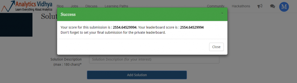
I never doubted GBM once. If done well, boosting algorithms usually pays off well. Now, will be interesting to see my leaderboard position:

This is a massive leaderboard jump! It’s like a freefall but safe landing from 122nd to 25th rank. Can we do better ? May be, we can. Let’s now use Deep Learning algorithm in H2O and try to improve this score.
Deep Learning in H2O
Let me give you a quick overview of deep learning. In deep learning algorithm, there exist 3 layers namely input layer, hidden layer and output layer. It works as follows:
- We feed the data to input layer.
- It then transmits the data to hidden layer. These hidden layer comprises of neurons. These neurons uses some function and assist in mapping non linear relationship among the variables.The hidden layers are user specified.
- Finally, these hidden layers delivers the output to output layer which then gives us the result.
Let’s implement this algorithm now.
#deep learning models
> system.time(
dlearning.model <- h2o.deeplearning(y = y.dep,
x = x.indep,
training_frame = train.h2o,
epoch = 60,
hidden = c(100,100),
activation = "Rectifier",
seed = 1122
)
)
# |===================================| 100%
# user system elapsed
# 0.83 0.05 129.69
It got executed even faster than GBM model. GBM took ~739 seconds. The parameter hidden instructs the algorithms to create 2 hidden layers of 100 neurons each. epoch is responsible for the number of passes on the train data to be carried out. Activation refers to the activation function to be used throughout the network.
Anyways, let’s check its performance.
> h2o.performance(dlearning.model)
H2ORegressionMetrics: deeplearning
** Reported on training data. **
MSE: 6215346
R2 : 0.7515775
Mean Residual Deviance : 6215346
We see further improvement in the R² metric as compared to GBM model. This suggests that deep learning model has successfully captured large chunk of unexplained variances in the model. Let’s make the predictions and check the final score.
#making predictions
> predict.dl2 <- as.data.frame(h2o.predict(dlearning.model, test.h2o))
#create a data frame and writing submission file
> sub_dlearning <- data.frame(User_ID = test$User_ID, Product_ID = test$Product_ID, Purchase = predict.dl2$predict)
> write.csv(sub_dlearning, file = "sub_dlearning_new.csv", row.names = F)
Let’s upload our final submission and check the score.


Though, my score improved but rank didn’t. So, finally we ended up at 25th rank by using little bit of feature engineering and lot of machine learning algorithms. I hope you enjoyed this journey from rank 154th to rank 25th. If you have followed me till here, I assume you’d be ready to go one step further.
What could you do to further improve this model ?
Actually, there are multiple things you can do. Here, I list them down:
- Do parameter tuning in GBM, Deep Learning and Random Forest.
- Use grid search for parameter tuning. H2O has a nice function h2o.grid to do this task
- Think of creating more features which can bring new information to the model.
- Finally, ensemble all the results to obtain a better model.
Try these steps at your end, and let me know in comments how did it turn out for you!
End Notes
I hope you enjoyed this journey with data.table and H2O. Once you become proficient at using these two packages, you’d be able to avoid a lot of obstacles which arises due to memory issues. In this article, I discussed the steps (with R codes) to implement model building using data.table and H2O. Even though, H2O itself can undertake data munging tasks, but I believe data.table is a much easy to use (syntax wise) option.
With this article, my intent was to get you started with data.table and H2O to build models. I am sure after this modeling practice you will become curious enough to take a step further and know more about these packages.
Did this article made you learn something new? Do write in the comments about your suggestions, experience or any feedback which could allow me to help you in a better way.


What's the possible best method to visualize a high dimensional data in radionics or genomics.. Any tutorial in R on high dimensional data including data reduction and data combination
Hey Declane, you can use principal component analysis to work on high dimensional data. Check this out: www.analyticsvidhya.com/blog/2016/03/practical-guide-principal-component-analysis-python/ For visualization on high dimensional data, check this out: http://www.analyticsvidhya.com/blog/2015/07/guide-data-visualization-r/ It consists of all possible forms of visualization which you can implement in R.
Really Good One ... Reading huge data is what people will say problem with R But this package resolve the same ...
Thanks !
Nice timing, yet again! The FB recruiting competition started on Kaggle just yesterday, with a > 1GB training set.
Glad to know! Wish you all the best for this competition. :)