Deep Learning for Computer Vision – Introduction to Convolution Neural Networks

Introduction

The power of artificial intelligence is beyond our imagination. We all know robots have already reached a testing phase in some of the powerful countries of the world. Governments, large companies are spending billions in developing this ultra-intelligence creature. The recent existence of robots have gained attention of many research houses across the world.

Does it excite you as well ? Personally for me, learning about robots & developments in AI started with a deep curiosity and excitement in me! Let’s learn about computer vision today.

The earliest research in computer vision started way back in 1950s. Since then, we have come a long way but still find ourselves far from the ultimate objective. But with neural networks and deep learning, we have become empowered like never before.

Applications of deep learning in vision have taken this technology to a different level and made sophisticated things like self-driven cars possible in near future. In this article, I will also introduce you to Convolution Neural Networks which form the crux of deep learning applications in computer vision.

Note: This article is inspired by Stanford’s Class on Visual Recognition. Understanding this article requires prior knowledge of Neural Networks. If you are new to neural networks, you can start here. Another useful resource on basics of deep learning can be found here.

You can also learn Convolutional neural Networks in a structured and comprehensive manner by enrolling in this free course: Convolutional Neural Networks (CNN) from Scratch

Table of Contents

1. Challenges in Computer Vision
2. Overview of Traditional Approaches
3. Review of Neural Networks Fundamentals
4. Introduction to Convolution Neural Networks
5. Case Study: Increasing power of of CNNs in IMAGENET competition
6. Implementing CNNs using GraphLab (Practical in Python)

1. Challenges in Computer Vision (CV)

As the name suggests, the aim of computer vision (CV) is to imitate the functionality of human eye and brain components responsible for your sense of sight.

Doing actions such as recognizing an animal, describing a view, differentiating among visible objects are really a cake-walk for humans. You’d be surprised to know that it took decades of research to discover and impart the ability of detecting an object to a computer with reasonable accuracy.

The field of computer vision has witnessed continual advancements in the past 5 years. One of the most stated advancement is Convolution Neural Networks (CNNs). Today, deep CNNs form the crux of most sophisticated fancy computer vision application, such as self-driving cars, auto-tagging of friends in our facebook pictures, facial security features, gesture recognition, automatic number plate recognition, etc.

Let’s get familiar with it a bit more:

Object detection is considered to be the most basic application of computer vision. Rest of the other developments in computer vision are achieved by making small enhancements on top of this. In real life, every time we(humans) open our eyes, we unconsciously detect objects.

Since it is super-intuitive for us, we fail to appreciate the key challenges involved when we try to design systems similar to our eye. Lets start by looking at some of the key roadblocks:

1. Variations in Viewpoint
   • The same object can have different positions and angles in an image depending on the relative position of the object and the observer.
   • There can also be different positions. For instance look at the following images:
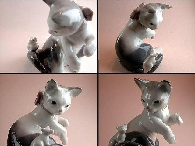
   • Though its obvious to know that these are the same object, it is not very easy to teach this aspect to a computer (robots or machines).
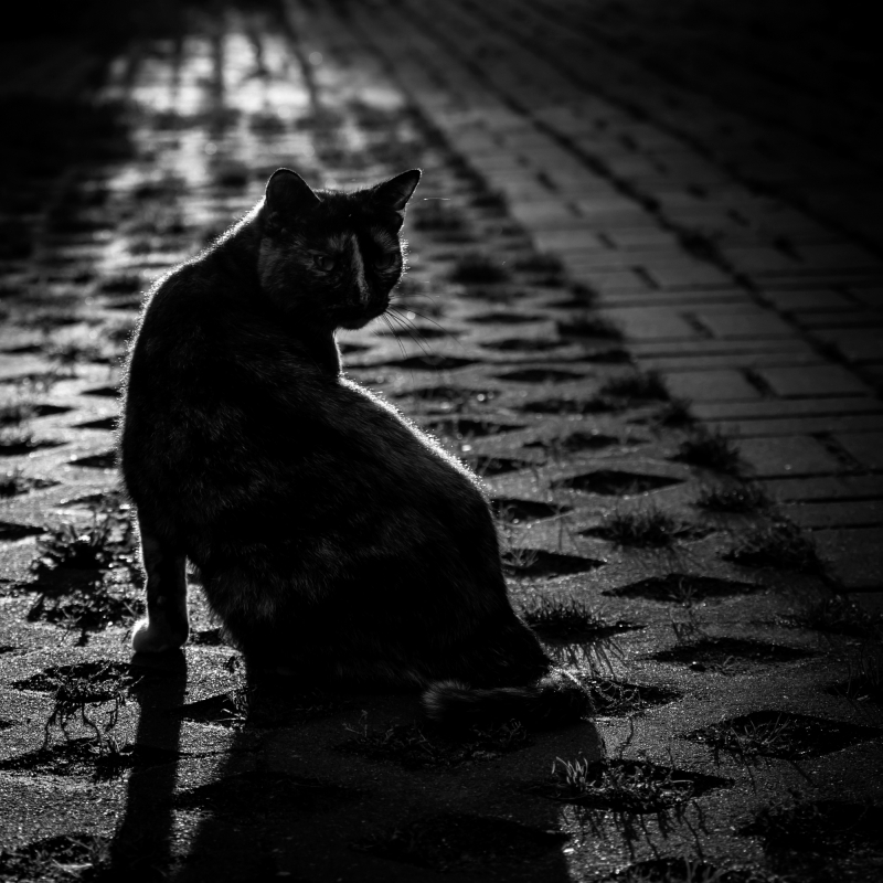
2. Difference in Illumination
   • Different images can have different light conditions. For instance:
     
   • Though this image is so dark, we can still recognize that it is a cat. Teaching this to a computer is another challenge.
3. Hidden parts of images
   • Images need not necessarily be complete. Small or large proportions of the images might be hidden which makes the detection task difficult. For instance:
     
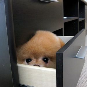
   • Here, only the face of the puppy is visible and that too partially, posing another challenge for the computer to recognize.
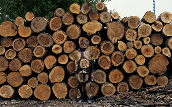
4. Background Clutter
   • Some images might blend into the background. For instance:
     
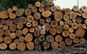
   • If you observe carefully, you can find a man in this image. As simple as it looks, it’s an uphill task for a computer to learn.

These are just some of the challenges which I brought up so that you can appreciate the complexity of the tasks which your eye and brain duo does with such utter ease. Breaking up all these challenges and solving individually is still possible today in computer vision. But we’re still decades away from a system which can get anywhere close to our human eye (which can do everything!).

This brilliance of our human body is the reason why researchers have been trying to break the enigma of computer vision by analyzing the visual mechanics of humans or other animals. Some of the earliest work in this direction was done by Hubel and Weisel with their famous cat experiment in 1959. Read more about it here.

This was the first study which emphasized the importance of edge detection for solving the computer vision problem. They were rewarded the nobel prize for their work.

Before diving into convolutional neural networks, lets take a quick overview of the traditional or rather elementary techniques used in computer vision before deep learning became popular.

2. Overview of Traditional Approaches

Various techniques, other than deep learning are available enhancing computer vision. Though, they work well for simpler problems, but as the data become huge and the task becomes complex, they are no substitute for deep CNNs. Let’s briefly discuss two simple approaches.

1. KNN (K-Nearest Neighbours)
   • Each image is matched with all images in training data. The top K with minimum distances are selected. The majority class of those top K is predicted as output class of the image.
   • Various distance metrics can be used like L1 distance (sum of absolute distance), L2 distance (sum of squares), etc.
   • Drawbacks:
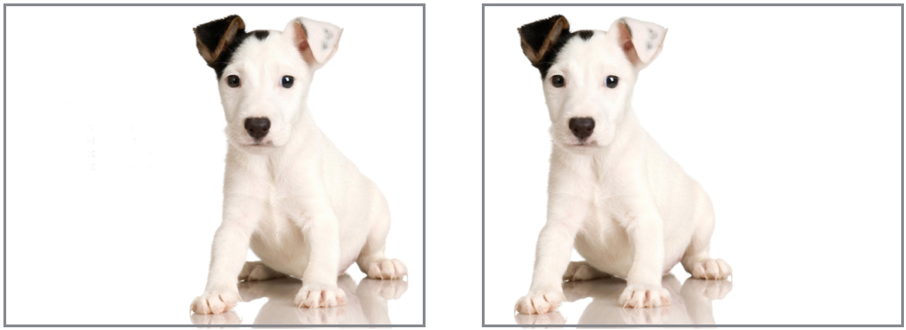
     • Even if we take the image of same object with same illumination and orientation, the object might lie in different locations of image, i.e. left, right or center of image. For instance:
       
     • Here the same dog is on right side in first image and left side in second. Though its the same image, KNN would give highly non-zero distance for the 2 images.
     • Similar to above, other challenges mentioned in section 1 will be faced by KNN.
2. Linear Classifiers
   • They use a parametric approach where each pixel value is considered as a parameter.
   • It’s like a weighted sum of the pixel values with the dimension of the weights matrix depending on the number of outcomes.
   • Intuitively, we can understand this in terms of a template. The weighted sum of pixels forms a template image which is matched with every image. This will also face difficulty in overcoming the challenges discussed in section 1 as single template is difficult to design for all the different cases.

I hope this gives some intuition into the challenges faced by approaches other than deep learning. Please note that more sophisticated techniques can be used than the ones discussed above but they would rarely beat a deep learning model.

3. Review of Neural Networks Fundamentals

Let’s discuss some properties of a neural networks. I will skip the basics of neural networks here as I have already covered that in my previous article – Fundamentals of Deep Learning – Starting with Neural Networks.

Once your fundamentals are sorted, let’s learn in detail some important concepts such as activation functions, data preprocessing, initializing weights and dropouts.

Activation Functions

There are various activation functions which can be used and this is an active area of research. Let’s discuss some of the popular options:

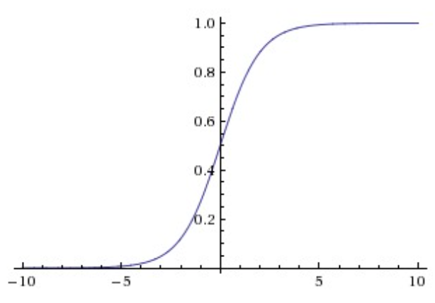
1. Sigmoid Function
   • Equation: σ(x) = 1/(1+e^-x)
     
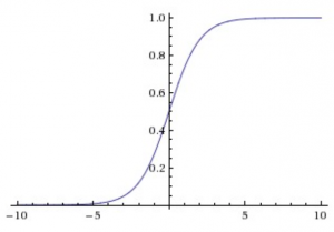
   • Sigmoid activation, also used in logistic regression regression, squashes the input space from (-inf,inf) to (0,1)
   • But it has various problems and it is almost never used in CNNs:
     1. Saturated neurons kill the gradient
        • If you observe the above graph carefully, if the input is beyond -5 or 5, the output will be very close to 0 and 1 respectively. Also, in this region the gradients are almost zero. Notice that the tangents in this region will be almost parallel to x-axis thus ~0 slope.
        • As we know that gradients get multiplied in back-propogation, so this small gradient will virtually stop back-propogation into further layers, thus killing the gradient.
     2. Outputs are not zero-centered
        • As you can see that all the outputs are between 0 and 1. As these become inputs to the next layer, all the gradients of the next layer will be either positive or negative. So the path to optimum will be zig-zag. I will skip the mathematics here. Please refer the stanford class referred above for details.
     3. Taking the exp() is computationally expensive
        • Though not a big drawback, it has a slight negative impact
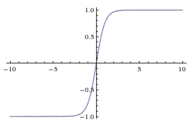
2. tanh activation
   • It is simply the hyperbolic tangent function with form:
     
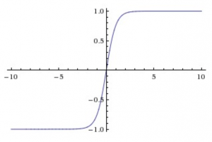
   • It is always preferred over sigmoid because it solved problem #2, i.e. the outputs are in range (-1,1).
   • But it will still result in killing the gradient and thus not recommended choice.
3.  ReLU (Rectified Linear Unit)
   • Equation: f(x) = max( 0 , x )
     
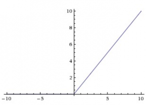
   • It is the most commonly used activation function for CNNs. It has following advantages:
     • Gradient won’t saturate in the positive region
     • Computationally very efficient as simple thresholding is required
     • Empirically found to converge faster than sigmoid or tanh.
   • But still it has the following disadvantages:
     • Output is not zero-centered and always positive
     • Gradient is killed for x<0. Few techniques like leaky ReLU and parametric ReLU are used to overcome this and I encourage you to find these
     • Gradient is not defined at x=0. But this can be easily catered using sub-gradients and posts less practical challenges as x=0 is generally a rare case

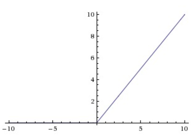
To summarize, ReLU is mostly the activation function of choice. If the caveats are kept in mind, these can be used very efficiently.

Data Preprocessing

For images, generally the following preprocessing steps are done:

1. Same Size Images: All images are converted to the same size and generally in square shape.
2. Mean Centering: For each pixel, its mean value among all images can be subtracted from each pixel. Sometimes (but rarely) mean centering along red, green and blue channels can also be done

Note that normalization is generally not done in images.

Weight Initialization

There can be various techniques for initializing weights. Lets consider a few of them:

1. All zeros
   • This is generally a bad idea because in this case all the neuron will generate the same output initially and similar gradients would flow back in back-propagation
   • The results are generally undesirable as network won’t train properly.
2. Gaussian Random Variables
   • The weights can be initialized with random gaussian distribution of 0 mean and small standard deviation (0.1 to 1e-5)
   • This works for shallow networks, i.e. ~5 hidden layers but not for deep networks
   • In case of deep networks, the small weights make the outputs small and as you move towards the end, the values become even smaller. Thus the gradients will also become small resulting in gradient killing at the end.
   • Note that you need to play with the standard deviation of the gaussian distribution which works well for your network.
3. Xavier Initialization
   • It suggests that variance of the gaussian distribution of weights for each neuron should depend on the number of inputs to the layer.
   • The recommended variance is square root of inputs. So the numpy code for initializing the weights of layer with n inputs is: np.random.randn(n_in, n_out)*sqrt(1/n_in)
   • A recent research suggested that for ReLU neurons, the recommended update is: np.random.randn(n_in, n_out)*sqrt(2/n_in). Read this blog post for more details.

One more thing must be remembered while using ReLU as activation function. It is that the weights initialization might be such that some of the neurons might not get activated because of negative input. This is something that should be checked. You might be surprised to know that 10-20% of the ReLUs might be dead at a particular time while training and even in the end.

These were just some of the concepts I discussed here. Some more concepts can be of importance like batch normalization, stochastic gradient descent, dropouts which I encourage you to read on your own.

4. Introduction to Convolution Neural Networks

Before going into the details, lets first try to get some intuition into why deep networks work better.

As we learned from the drawbacks of earlier approaches, they are unable to cater to the vast amount of variations in images. Deep CNNs work by consecutively modeling small pieces of information and combining them deeper in network.

One way to understand them is that the first layer will try to detect edges and form templates for edge detection. Then subsequent layers will try to combine them into simpler shapes and eventually into templates of different object positions, illumination, scales, etc. The final layers will match an input image with all the templates and the final prediction is like a weighted sum of all of them. So, deep CNNs are able to model complex variations and behaviour giving highly accurate predictions.

There is an interesting paper on visualization of deep features in CNNs which you can go through to get more intuition – Understanding Neural Networks Through Deep Visualization.

For the purpose of explaining CNNs and finally showing an example, I will be using the CIFAR-10 dataset for explanation here and you can download the data set from here. This dataset has 60,000 images with 10 labels and 6,000 images of each type. Each image is colored and 32×32 in size.

A CNN typically consists of 3 types of layers:

1. Convolution Layer
2. Pooling Layer
3. Fully Connected Layer

You might find some batch normalization layers in some old CNNs but they are not used these days. We’ll consider these one by one.

Convolution Layer

Since convolution layers form the crux of the network, I’ll consider them first. Each layer can be visualized in the form of a block or a cuboid. For instance in the case of CIFAR-10 data, the input layer would have the following form:

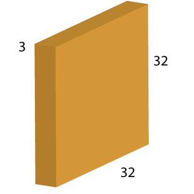
Here you can see, this is the original image which is 32×32 in height and width. The depth here is 3 which corresponds to the Red, Green and Blue colors, which form the basis of colored images. Now a convolution layer is formed by running a filter over it. A filter is another block or cuboid of smaller height and width but same depth which is swept over this base block. Let’s consider a filter of size 5x5x3.

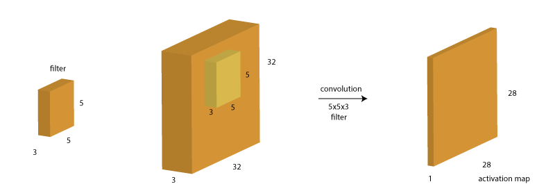
We start this filter from the top left corner and sweep it till the bottom left corner. This filter is nothing but a set of eights, i.e. 5x5x3=75 + 1 bias = 76 weights. At each position, the weighted sum of the pixels is calculated as W^TX + b and a new value is obtained. A single filter will result in a volume of size 28x28x1 as shown above.

Note that multiple filters are generally run at each step. Therefore, if 10 filters are used, the output would look like:

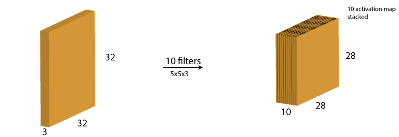
Here the filter weights are parameters which are learned during the back-propagation step. You might have noticed that we got a 28×28 block as output when the input was 32×32. Why so? Let’s look at a simpler case.

Suppose the initial image had size 6x6xd and the filter has size 3x3xd. Here I’ve kept the depth as d because it can be anything and it’s immaterial as it remains the same in both. Since depth is same, we can have a look at the front view of how filter would work:

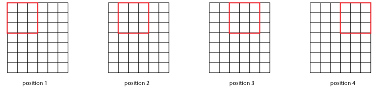
Here we can see that the result would be 4x4x1 volume block. Notice there is a single output for entire depth of the each location of filter. But you need not do this visualization all the time. Let’s define a generic case where image has dimension NxNxd and filter has FxFxd. Also, lets define another term stride (S) here which is the number of cells (in above matrix) to move in each step. In the above case, we had a stride of 1 but it can be a higher value as well. So the size of the output will be:

output size = (N – F)/S + 1

You can validate the first case where N=32, F=5, S=1. The output had 28 pixels which is what we get from this formula as well. Please note that some S values might result in non-integer result and we generally don’t use such values.

Let’s consider an example to consolidate our understanding. Starting with the same image as before of size 32×32, we need to apply 2 filters consecutively, first 10 filters of size 7, stride 1 and next 6 filters of size 5, stride 2. Before looking at the solution below, just think about 2 things:

1. What should be the depth of each filter?
2. What will the resulting size of the images in each step.

Here is the answer:

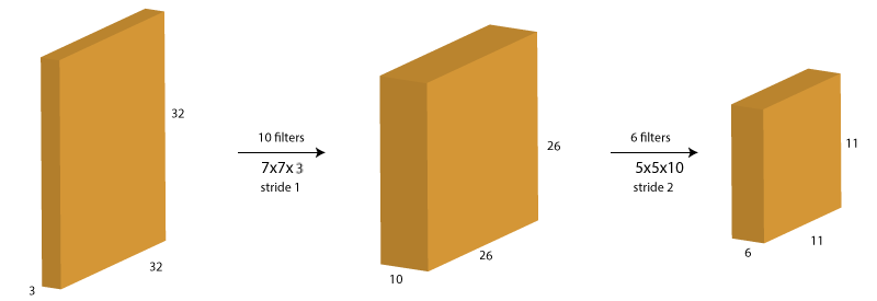
Notice here that the size of the images is getting shrunk consecutively. This will be undesirable in case of deep networks where the size would become very small too early. Also, it would restrict the use of large size filters as they would result in faster size reduction.

To prevent this, we generally use a stride of 1 along with zero-padding of size (F-1)/2. Zero-padding is nothing but adding additional zero-value pixels towards the border of the image.

Consider the example we saw above with 6×6 image and 3×3 filter. The required padding is (3-1)/2=1. We can visualize the padding as:

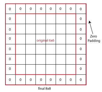
Here you can see that the image now becomes 8×8 because of padding of 1 on each side. So now the output will be of size 6×6 same as the original image.

Now let’s summarize a convolution layer as following:

• Input size: W₁ x H₁ x D₁
• Hyper-parameters:
  • K: #filters
  • F: filter size (FxF)
  • S: stride
  • P: amount of padding
• Output size: W₂ x H₂ x D₂
  • W₂₁
  • H₂₁
  • D₂
• #parameters = (F.F.D).K + K
  • F.F.D : Number of parameters for each filter (analogous to volume of the cuboid)
  • (F.F.D).K : Volume of each filter multiplied by the number of filters
  • +K: adding K parameters for the bias term

Some additional points to be taken into consideration:

• K should be set as powers of 2 for computational efficiency
• F is generally taken as odd number
• F=1 might sometimes be used and it makes sense because there is a depth component involved
• Filters might be called kernels sometimes

Having understood the convolution layer, lets move on to pooling layer.

Pooling Layer

When we use padding in convolution layer, the image size remains same. So, pooling layers are used to reduce the size of image. They work by sampling in each layer using filters. Consider the following 4×4 layer. So if we use a 2×2 filter with stride 2 and max-pooling, we get the following response:

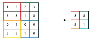
Here you can see that 4 2×2 matrix are combined into 1 and their maximum value is taken. Generally, max-pooling is used but other options like average pooling can be considered.

Fully Connected Layer

At the end of convolution and pooling layers, networks generally use fully-connected layers in which each pixel is considered as a separate neuron just like a regular neural network. The last fully-connected layer will contain as many neurons as the number of classes to be predicted. For instance, in CIFAR-10 case, the last fully-connected layer will have 10 neurons.

5. Case Study: AlexNet

I recommend reading the prior section multiple times and getting a hang of the concepts before moving forward.

In this section, I will discuss the AlexNet architecture in detail. To give you some background, AlexNet is the winning solution of IMAGENET Challenge 2012. This is one of the most reputed computer vision challenge and 2012 was the first time that a deep learning network was used for solving this problem.

Also, this resulted in a significantly better result as compared to previous solutions. I will share the network architecture here and review all the concepts learned above.

The detailed solution has been explained in this paper. I will explain the overall architecture of the network here. The AlexNet consists of a 11 layer CNN with the following architecture:

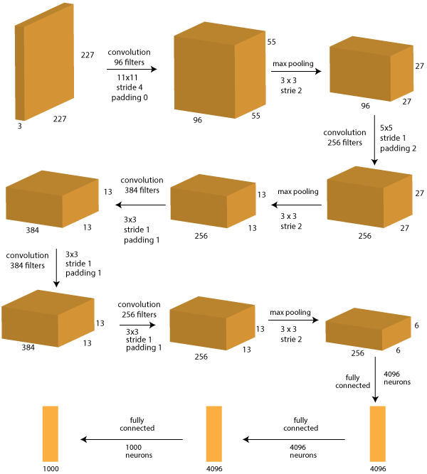
Here you can see 11 layers between input and output. Lets discuss each one of them individually. Note that the output of each layer will be the input of next layer. So you should keep that in mind.

• Layer 0: Input image
  • Size: 227 x 227 x 3
  • Note that in the paper referenced above, the network diagram has 224x224x3 printed which appears to be a typo.
• Layer 1: Convolution with 96 filters, size 11×11, stride 4, padding 0
  • Size: 55 x 55 x 96
  • (227-11)/4 + 1 = 55 is the size of the outcome
  • 96 depth because 1 set denotes 1 filter and there are 96 filters
• Layer 2: Max-Pooling with 3×3 filter, stride 2
  • Size: 27 x 27 x 96
  • (55 – 3)/2 + 1 = 27 is size of outcome
  • depth is same as before, i.e. 96 because pooling is done independently on each layer
• Layer 3: Convolution with 256 filters, size 5×5, stride 1, padding 2
  • Size: 27 x 27 x 256
  • Because of padding of (5-1)/2=2, the original size is restored
  • 256 depth because of 256 filters
• Layer 4: Max-Pooling with 3×3 filter, stride 2
  • Size: 13 x 13 x 256
  • (27 – 3)/2 + 1 = 13 is size of outcome
  • Depth is same as before, i.e. 256 because pooling is done independently on each layer
• Layer 5: Convolution with 384 filters, size 3×3, stride 1, padding 1
  • Size: 13 x 13 x 384
  • Because of padding of (3-1)/2=1, the original size is restored
  • 384 depth because of 384 filters
• Layer 6: Convolution with 384 filters, size 3×3, stride 1, padding 1
  • Size: 13 x 13 x 384
  • Because of padding of (3-1)/2=1, the original size is restored
  • 384 depth because of 384 filters
• Layer 7: Convolution with 256 filters, size 3×3, stride 1, padding 1
  • Size: 13 x 13 x 256
  • Because of padding of (3-1)/2=1, the original size is restored
  • 256 depth because of 256 filters
• Layer 8: Max-Pooling with 3×3 filter, stride 2
  • Size: 6 x 6 x 256
  • (13 – 3)/2 + 1 = 6 is size of outcome
  • Depth is same as before, i.e. 256 because pooling is done independently on each layer
• Layer 9: Fully Connected with 4096 neuron
  • In this later, each of the 6x6x256=9216 pixels are fed into each of the 4096 neurons and weights determined by back-propagation.
• Layer 10: Fully Connected with 4096 neuron
  • Similar to layer #9
• Layer 11: Fully Connected with 1000 neurons
  • This is the last layer and has 1000 neurons because IMAGENET data has 1000 classes to be predicted.

I understand this is a complicated structure but once you understand the layers, it’ll give you a much better understanding of the architecture. Note that you fill find a different representation of the structure if you look at the AlexNet paper. This is because at that GPUs were not very powerful and they used 2 GPUs for training the network. So the work processing was divided between the two.

I highly encourage you to go through the other advanced solutions of ImageNet challenges after 2012 to get more ideas of how people design these networks. Some of interesting solutions are:

• ZFNet: winner of 2013 challenge
• GoogleNet: winner of 2014 challenge
• VGGNet: a good solution from 2014 challenge
• ResNet: winner of 2015 challenge designed by Microsoft Research Team

This video gives a brief overview and comparison of these solutions towards the end.

6. Implementing CNNs using GraphLab

Having understood the theoretical concepts, lets move on to the fun part (practical) and make a basic CNN on the CIFAR-10 dataset which we’ve downloaded before.

I’ll be using GraphLab for the purpose of running algorithms. Instead of GraphLab, you are free to use alternatives tools such as Torch, Theano, Keras, Caffe, TensorFlow, etc. But GraphLab allows a quick and dirty implementation as it takes care of the weights initializations and network architecture on its own.

We’ll work on the CIFAR-10 dataset which you can download from here. The first step is to load the data. This data is packed in a specific format which can be loaded using the following code:

import pandas as pd
import numpy as np
import cPickle

#Define a function to load each batch as dictionary:
def unpickle(file):
    fo = open(file, 'rb')
    dict = cPickle.load(fo)
    fo.close()
    return dict

#Make dictionaries by calling the above function:
batch1 = unpickle('data/data_batch_1')
batch2 = unpickle('data/data_batch_2')
batch3 = unpickle('data/data_batch_3')
batch4 = unpickle('data/data_batch_4')
batch5 = unpickle('data/data_batch_5')
batch_test = unpickle('data/test_batch')

#Define a function to convert this dictionary into dataframe with image pixel array and labels:
def get_dataframe(batch):
    df = pd.DataFrame(batch['data'])
    df['image'] = df.as_matrix().tolist()
    df.drop(range(3072),axis=1,inplace=True)
    df['label'] = batch['labels']
    return df

#Define train and test files:
train = pd.concat([get_dataframe(batch1),get_dataframe(batch2),get_dataframe(batch3),get_dataframe(batch4),get_dataframe(batch5)],ignore_index=True)
test = get_dataframe(batch_test)

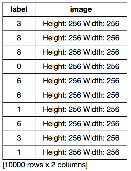
We can verify this data by looking at the head and shape of data as follow:

print train.head()

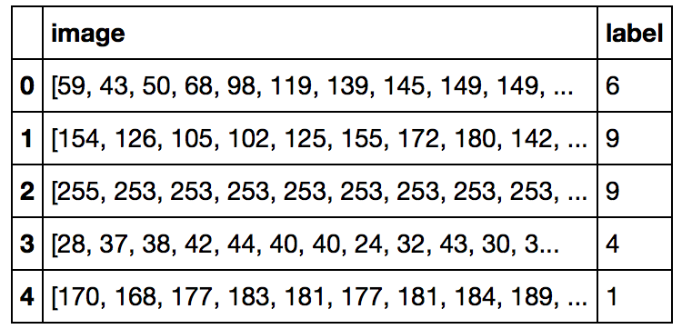
print train.shape, test.shape

Since we’ll be using graphlab, the next step is to convert this into a graphlab SFrame and run neural network. Let’s convert the data first:

import graphlab as gl
gltrain = gl.SFrame(train)
gltest = gl.SFrame(test)

GraphLab has a functionality of automatically creating a neural network based on the data. Lets run that as a baseline model before going into an advanced model.

model = gl.neuralnet_classifier.create(gltrain, target='label', validation_set=None)

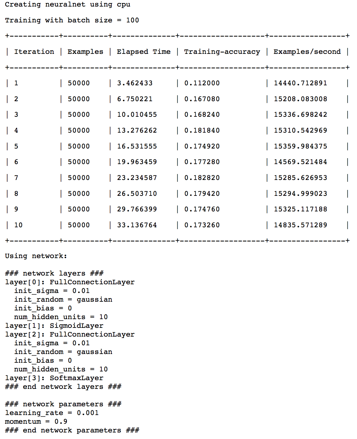
Here it used a simple fully connected network with 2 hidden layers and 10 neurons each. Let’s evaluate this model on test data.

model.evaluate(gltest)

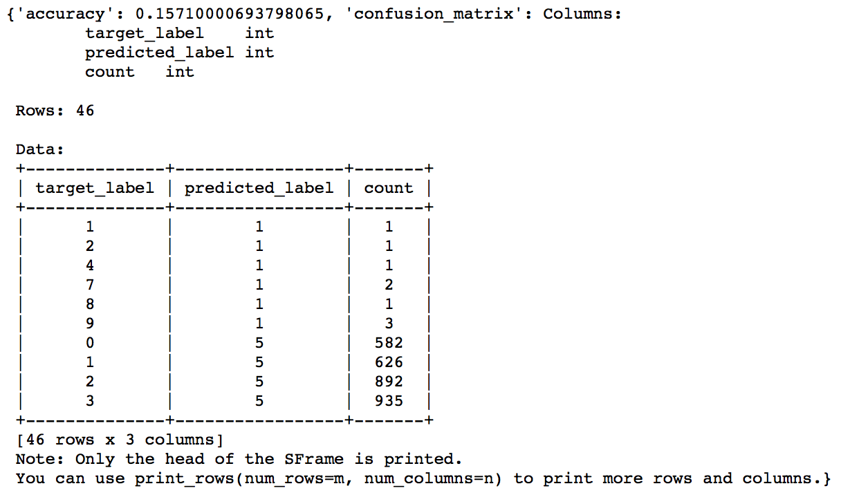
As you can see that we have a pretty low accuracy of ~15%. This is because it is a very fundamental network. Lets try to make a CNN now. But if we go about training a deep CNN from scratch, we will face the following challenges:

1. The available data is very less to capture all the required features
2. Training deep CNNs generally requires a GPU as a CPU is not powerful enough to perform the required calculations. Thus we won’t be able to run it on our system. We can probably rent an Amazom AWS instance.

To overcome these challenges, we can use pre-trained networks. These are nothing but networks like AlexNet which are pre-trained on many images and the weights for deep layers have been determined. The only challenge is to find a pre-trianed network which has been trained on images similar to the one we want to train. If the pre-trained network is not made on images of similar domain, then the features will not exactly make sense and classifier will not be of higher accuracy.

Before proceeding further, we need to convert these images into the size used in ImageNet which we’re using for classification. The GraphLab model is based on 256×256 size images. So we need to convert our images to that size. Lets do it using the following code:

#Convert pixels to graphlab image format
gltrain['glimage'] = gl.SArray(gltrain['image']).pixel_array_to_image(32, 32, 3, allow_rounding = True)
gltest['glimage'] = gl.SArray(gltest['image']).pixel_array_to_image(32, 32, 3, allow_rounding = True)

#Remove the original column
gltrain.remove_column('image')
gltest.remove_column('image')

gltrain.head()

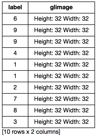
Here we can see that a new column of type graphlab image has been created but the images are in 32×32 size. So we convert them to 256×256 using following code:

#Convert into 256x256 size
gltrain['image'] = gl.image_analysis.resize(gltrain['glimage'], 256, 256, 3)
gltest['image'] = gl.image_analysis.resize(gltest['glimage'], 256, 256, 3)

#Remove old column:
gltrain.remove_column('glimage')
gltest.remove_column('glimage')

gltrain.head()

Now we can see that the image has been converted into the desired size. Next, we will load the ImageNet pre-trained model in graphlab and use the features created in its last layer into a simple classifier and make predictions.

Lets start by loading the pre-trained model.

#Load the pre-trained model:
pretrained_model = gl.load_model('http://s3.amazonaws.com/GraphLab-Datasets/deeplearning/imagenet_model_iter45')

Now we have to use this model and extract features which will be passed into a classifier. Note that the following operations may take a lot of computing time. I use a Macbook Pro 15″ and I had to leave it for whole night!

gltrain['features'] = pretrained_model.extract_features(gltrain)
gltest['features'] = pretrained_model.extract_features(gltest)

Lets have a look at the data to make sure we have the features:

gltrain.head()

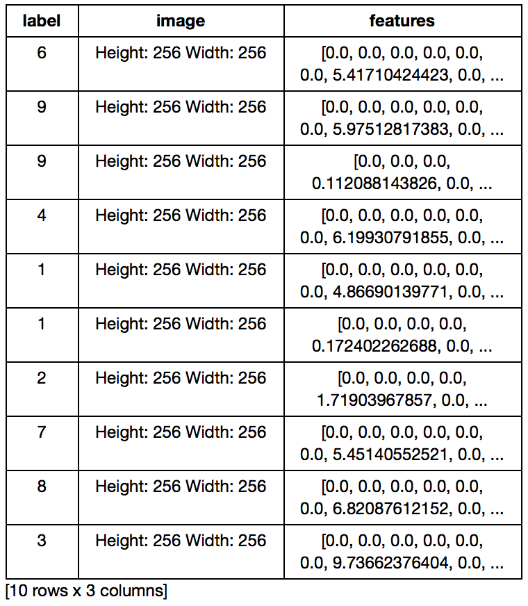
Though, we have the features with us, notice here that lot of them are zeros. You can understand this as a result of smaller data set. ImageNet was created on 1.2Mn images. So there would be many features in those images that don’t make sense for this data, thus resulting in zero outcome.

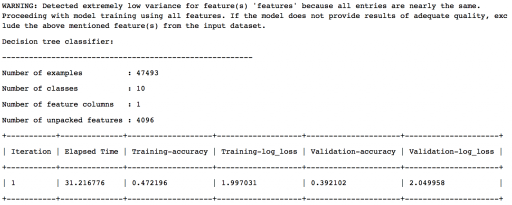
Now lets create a classifier using graphlab. The advantage with “classifier” function is that it will automatically create various classifiers and chose the best model.

simple_classifier = graphlab.classifier.create(gltrain, features = ['features'], target = 'label')

The various outputs are:

1. Boosted Trees Classifier
   
2. Random Forest Classifier
   
   
3. Decision Tree Classifier
   
   
4. Logistic Regression Classifier
   

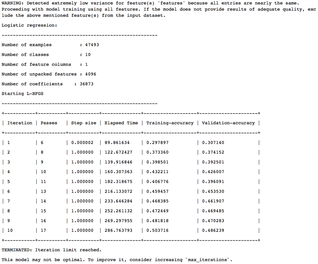
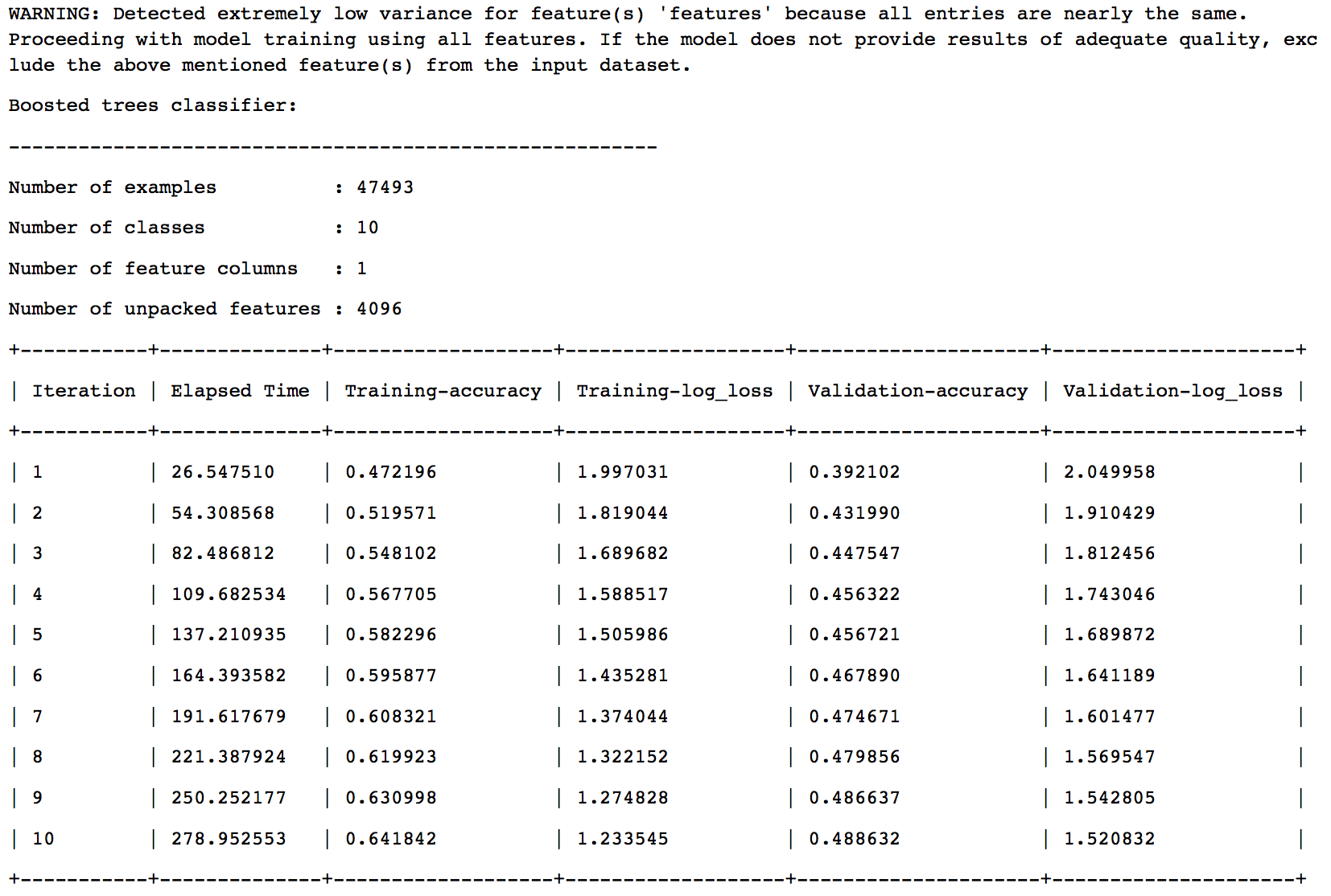
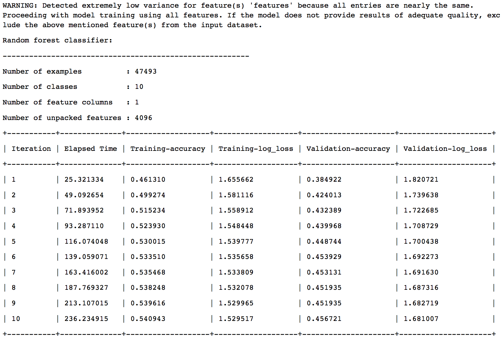
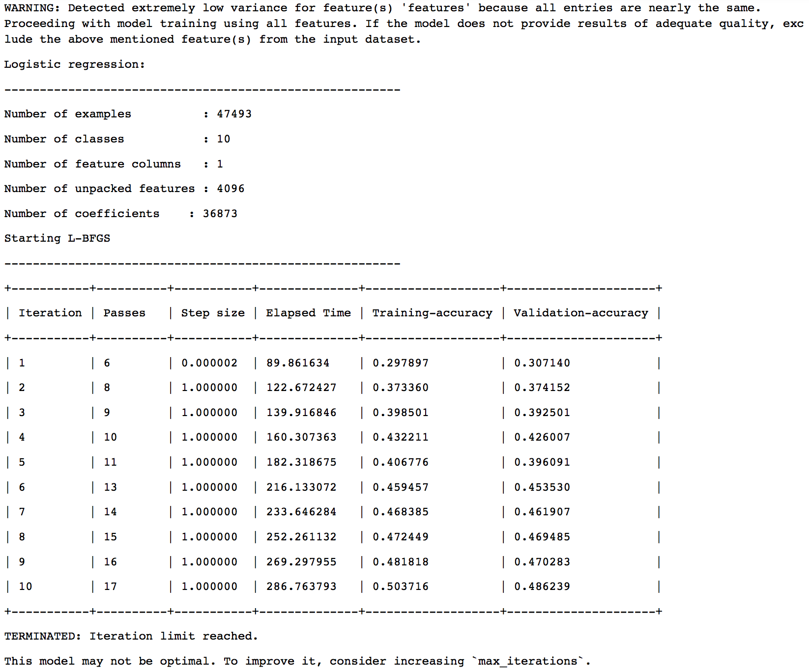
The final model selection is based on a validation set with 5% of the data. The results are:

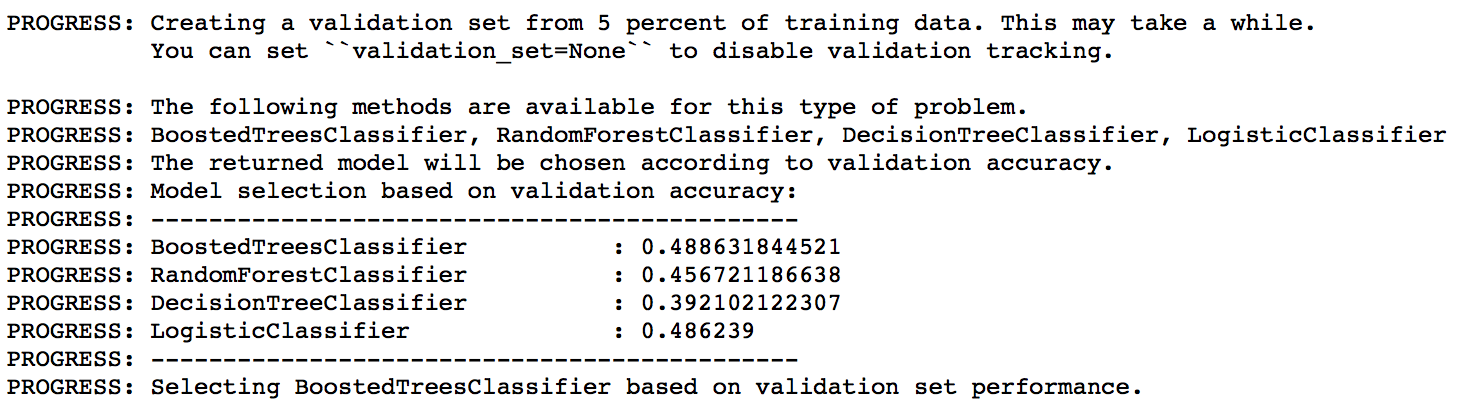
So we can see that Boosted Trees Classifier has been chosen as the final model. Let’s look at the results on test data:

simple_classifier.evaluate(gltest)

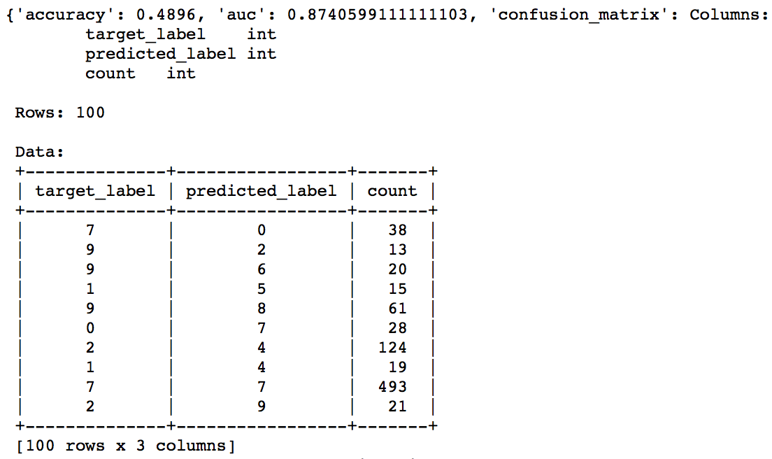
So we can see that the test accuracy is now ~50%. It’s a decent jump from 15% to 50% but there is still huge potential to do better. The idea here was to get you started and I will skip the next steps. Here are some things which you can try:

1. Remove the redundant features in the data
2. Perform hyper-parameter tuning in models
3. Search for pre-trained models which are trained on images similar to this dataset

You can find many open-source solutions for this dataset which give >95% accuracy. You should check those out. Please feel free to try them and post your solutions in comments below.

Projects

Now, its time to take the plunge and actually play with some other real datasets. So are you ready to take on the challenge? Accelerate your deep learning journey with the following Practice Problems:

	Practice Problem: Identify the Apparels	Identify the type of apparel for given images
	Practice Problem: Identify the Digits	Identify the digit in given images

End Notes

In this article, we covered the basics of computer vision using deep Convolution Neural Networks (CNNs). We started by appreciating the challenges involved in designing artificial systems which mimic the eye. Then, we looked at some of the traditional techniques, prior to deep learning, and got some intuition into their drawbacks.

We moved on to understanding the some aspects of tuning a neural networks such as activation functions, weights initialization and data-preprocessing. Next, we got some intuition into why deep CNNs should work better than traditional approaches and we understood the different elements present in a general deep CNN.

Subsequently, we consolidated our understanding by analyzing the architecture of AlexNet, the winning solution of ImageNet 2012 challenge. Finally, we took the CIFAR-10 data and implemented a CNN on it using a pre-trained AlexNet deep network.

I hope you liked this article. Did you find this article useful ? Please feel free to share your feedback through comments below. And to gain expertise in working in neural network try out the deep learning practice problem – Identify the Digits.

You can test your skills and knowledge. Check out Live Competitions and compete with best Data Scientists from all over the world.

Aarshay Jain

Aarshay graduated from MS in Data Science at Columbia University in 2017 and is currently an ML Engineer at Spotify New York. He works at an intersection or applied research and engineering while designing ML solutions to move product metrics in the required direction. He specializes in designing ML system architecture, developing offline models and deploying them in production for both batch and real time prediction use cases.