Introduction
It is often said that in machine learning (and more specifically deep learning) – it’s not the person with the best algorithm that wins, but the one with the most data. We can always try and collect or generate more labelled data but it’s an expensive and time consuming task.
This is where the promise and potential of unsupervised deep learning algorithms comes into the picture. They are designed to derive insights from the data without any supervision. For example, customers can be segmented into different groups based on their buying behaviour. This information can then be used to serve up better product recommendations.
In my previous article “Essentials of Deep Learning: Introduction to Unsupervised Deep Learning“, I gave you a high level overview of what unsupervised deep learning is, and it’s potential applications.
In this article, we will explore different algorithms, which fall in the category of unsupervised deep learning. We will go through them one-by-one using a computer vision problem to understand how they work and how they can be used in practical applications.
Note: This article assumes familiarity with Deep Learning. You can go through the below articles to get an overview:
- Fundamentals of Deep Learning – Starting with Artificial Neural Network
- Tutorial: Optimizing Neural Networks using Keras (with Image recognition case study)
Table of Contents
- Building Blocks of Unsupervised Deep Learning
- Exploring Unsupervised Deep Learning algorithms on Fashion MNIST dataset
- Image Reconstruction using a simple AutoEncoder
- Sparse Image Compression using Sparse AutoEncoders
- Image Denoising using Denoising AutoEncoders
- Image Generation using Variational AutoEncoder
Building Blocks of Unsupervised Deep Learning – AutoEncoders
Let’s do a quick refresher on the concept of AutoEncoder. There are two important concepts of an AutoEncoder, which makes it a very powerful algorithm for unsupervised learning problems:
- They try to produce an output which is extremely similar to the given input
- They generally have an hourglass like shape, i.e., they have a bottleneck in between the encoder and the decoder model
We will take an example of an AutoEncoder trained on images of cats, each of size 100×100. So the input dimension is 10,000, and the AutoEncoder has to represent all this information in a vector of size 10, which makes the model learn only the important parts of the images so that it can re-create the original image just from this vector.
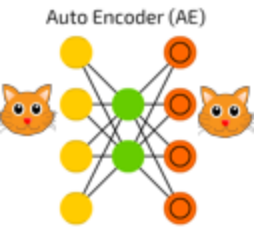
An autoencoder can be logically divided into two parts: an encoder part and a decoder part. The task of the encoder is to convert the input to a lower dimensional representation, while the task of the decoder is to recreate the input from this lower dimensional representation.
Let us get a more practical perspective on these algorithms by implementing them on a real life problem.
Note – This article is heavily influenced by Francois Chollet’s tutorial. Special thanks to him for an excellent roundup!
Exploring Unsupervised Deep Learning algorithms on Fashion MNIST dataset
Before we dive on to the implementations, let us take a minute to understand our dataset, aka Fashion MNIST, which is a problem of apparel recognition. Fashion is a broad field that is seeming a huge boom thanks in large part to the power of machine learning. Seems like an appropriate challenge to learn a technique!
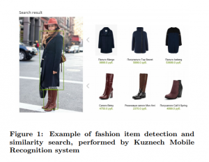
Source: KDDFashion
In this problem, we need to identify the type of apparel in a set of images. We have a total of 70,000 images, out of which 60,000 are a part of train images with the label of the type of apparel (total classes: 10) and the remaining 10,000 images are unlabelled (known as test images).
| Label | Description |
| 0 | T-shirt/top |
| 1 | Trouser |
| 2 | Pullover |
| 3 | Dress |
| 4 | Coat |
| 5 | Sandal |
| 6 | Shirt |
| 7 | Sneaker |
| 8 | Bag |
| 9 | Ankle boot |
In our experiments below, we will ignore the labels, and only work on the training images in an unsupervised way. A potential use case of applying unsupervised learning on this dataset is suggesting similar fashion items that the person may like.
Image Reconstruction using a simple AutoEncoder
Now that we know what an autoencoder is, we will apply it on a problem to understand how we can leverage it for real life applications. A straight-forward task could be to compress a given image into discrete bits of information, and reconstruct the image back from these discrete bits.
A typical use-case could be to transfer images from one location to another, and using it to lower bandwidth.
To work on the problem, we will first have to load all the necessary libraries. We will be coding in python, and will build neural network models in keras. So make sure you have set up your system before reading further. Otherwise you can refer to the official installation guide to install keras.
In [1]:
from keras.datasets import fashion_mnist
In [2]:
%pylab inline
import os
import keras
import numpy as np
import pandas as pd
import keras.backend as K

from time import time
from sklearn.cluster import KMeans
from keras import callbacks
from keras.models import Model
from keras.optimizers import SGD
from keras.layers import Dense, Input
from keras.initializers import VarianceScaling
from keras.engine.topology import Layer, InputSpec

from scipy.misc import imread
from sklearn.metrics import accuracy_score, normalized_mutual_info_score
Now download the image data and read it in numpy format.
In [3]:
(train_x, train_y), (val_x, val_y) = fashion_mnist.load_data()
We will do the required pre-processing on our data, so that we can push it through our neural network model.
train_x = train_x/255.
val_x = val_x/255.

train_x = train_x.reshape(-1, 784)
val_x = val_x.reshape(-1, 784)
Now let’s define the autoencoder model.
In [11]:
# this is our input placeholder
input_img = Input(shape=(784,))

# "encoded" is the encoded representation of the input
encoded = Dense(2000, activation='relu')(input_img)
encoded = Dense(500, activation='relu')(encoded)
encoded = Dense(500, activation='relu')(encoded)
encoded = Dense(10, activation='sigmoid')(encoded)

# "decoded" is the lossy reconstruction of the input
decoded = Dense(500, activation='relu')(encoded)
decoded = Dense(500, activation='relu')(decoded)
decoded = Dense(2000, activation='relu')(decoded)
decoded = Dense(784)(decoded)

# this model maps an input to its reconstruction
autoencoder = Model(input_img, decoded)
Here is how our model looks like:
In [12]:
autoencoder.summary()
We will then compile and run our autoencoder model:
In [13]:
#  this model maps an input to its encoded representation
encoder = Model(input_img, encoded)
In [14]:
autoencoder.compile(optimizer='adam', loss='mse')
In [15]:
estop = keras.callbacks.EarlyStopping(monitor='val_loss', min_delta=0, patience=10, verbose=1, mode='auto')
In [17]:
train_history = autoencoder.fit(train_x, train_x, epochs=500, batch_size=2048, validation_data=(val_x, val_x), callbacks=[estop])
Now that our model is trained, it’s time for predictions!
In [19]:
pred = autoencoder.predict(val_x)
Here is how our predicted image looks like:
In [24]:
plt.imshow(pred[0].reshape(28, 28), cmap='gray')
Out[24]:

Let’s print the original image just to see the comparison.
In [25]:
plt.imshow(val_x[0].reshape(28, 28), cmap='gray')
Out[25]:

On comparing this with the original image, looks like our model gives us a good enough reconstruction.
Sparse Image Compression using a Sparse AutoEncoder
Now that we know how to reconstruct an image, we will see how we can improve our model.
For our use case of sending an image from one location to another, we used the output of 10 neurons for compressing the image. An optimization on this we can do is to make this representation sparse, so that we require even less bits than we needed before to transfer the compressed image properties and reconstruct it back to the original image at the other end.
This can be done using a modified autoencoder called sparse autoencoder. Technically speaking, to make representations more compact, we add a sparsity constraint on the activity of the hidden representations (called activity regularizer in keras), so that fewer units get activated at a given time to give us an optimal reconstruction.
Ready to go on? Now we will see how we can create a sparse autoencoder model. We will redo all the steps again, but with a small change in how we create our model network.
from keras.datasets import fashion_mnist
In [2]:
%pylab inline
import os
import keras
import numpy as np
import pandas as pd
import keras.backend as K
from keras import regularizers


from time import time
from sklearn.cluster import KMeans
from keras import callbacks
from keras.models import Model
from keras.optimizers import SGD
from keras.layers import Dense, Input
from keras.initializers import VarianceScaling
from keras.engine.topology import Layer, InputSpec

from scipy.misc import imread
from sklearn.metrics import accuracy_score, normalized_mutual_info_score
In [3]:
(train_x, train_y), (val_x, val_y) = fashion_mnist.load_data()
In [4]:
train_x = train_x/255.
val_x = val_x/255.

train_x = train_x.reshape(-1, 784)
val_x = val_x.reshape(-1, 784)
When we create our model, we add an activity constraint by defining a small value in the activity_regularizer argument.
In [5]:
# this is our input placeholder
input_img = Input(shape=(784,))

# "encoded" is the encoded representation of the input
encoded = Dense(2000, activation='relu')(input_img)
encoded = Dense(500, activation='relu',
                activity_regularizer=regularizers.l1(10e-10))(encoded)
encoded = Dense(500, activation='relu',
                activity_regularizer=regularizers.l1(10e-10))(encoded)
encoded = Dense(10, activation='sigmoid',
                activity_regularizer=regularizers.l1(10e-10))(encoded)

# "decoded" is the lossy reconstruction of the input
decoded = Dense(500, activation='relu')(encoded)
decoded = Dense(500, activation='relu')(decoded)
decoded = Dense(2000, activation='relu')(decoded)
decoded = Dense(784)(decoded)

# this model maps an input to its reconstruction
autoencoder = Model(input_img, decoded)
In [6]:
autoencoder.summary()
In [7]:
#  this model maps an input to its encoded representation
encoder = Model(input_img, encoded)
In [8]:
autoencoder.compile(optimizer='adam', loss='mse')
In [9]:
estop = keras.callbacks.EarlyStopping(monitor='val_loss', min_delta=0, patience=10, verbose=1, mode='auto')
In [10]:
train_history = autoencoder.fit(train_x, train_x, epochs=200, batch_size=2048, validation_data=(val_x, val_x), callbacks=[estop])
In [11]:
pred = autoencoder.predict(val_x)
In [12]:
plt.imshow(pred[0].reshape(28, 28), cmap='gray')
Out[12]:

In [13]:
plt.imshow(val_x[0].reshape(28, 28), cmap='gray')
Out[13]:
We see that our model performs almost similar to our vanilla autoencoder. But on inspecting the output of the encoder model, we can see that it uses much more sparse information to represent the original image.
Image Denoising with Denoising AutoEncoders
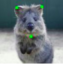
In this section, we’ll look at another potential application of autoencoders, i.e. image denoising. To understand this better, let us go through a graphical representation of this problem.
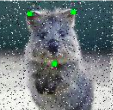
Suppose that our image gets corrupted, or there is a bit of noise in the image. In such a scenario, there is no straight-forward way to remove the noise. In image processing terms, we define this problem as an image denoising problem. What we need, is to convert this noisy image into a somewhat clearer image that has most (if not all) of the noise removed.
Now that we have an essence of what our problem is, let’s use deep autoencoders to solve the problem. Technically, there is not much difference in our model architecture – as we will see it in the implementation below. The difference is in the problem that our model is trying to solve, and the inputs and outputs.
from keras.datasets import fashion_mnist
In [2]:
%pylab inline
import os
import keras
import numpy as np
import pandas as pd
import keras.backend as K

from time import time
from sklearn.cluster import KMeans
from keras import callbacks
from keras.models import Model
from keras.optimizers import SGD
from keras.layers import Dense, Input, Conv2D, MaxPool2D, UpSampling2D
from keras.initializers import VarianceScaling
from keras.engine.topology import Layer, InputSpec

from scipy.misc import imread
from sklearn.metrics import accuracy_score, normalized_mutual_info_score
In [3]:
(train_x, train_y), (val_x, val_y) = fashion_mnist.load_data()
Here we will augment our input image in order to deliberately induce noise.
In [4]:
from imgaug import augmenters as iaa
seq = iaa.Sequential([iaa.SaltAndPepper(0.2)])

train_x_aug = seq.augment_images(train_x)
val_x_aug = seq.augment_images(val_x)
In [5]:
train_x = train_x/255.
val_x = val_x/255.

train_x = train_x.reshape(-1, 28, 28, 1)
val_x = val_x.reshape(-1, 28, 28, 1)

train_x_aug = train_x_aug/255.
val_x_aug = val_x_aug/255.

train_x_aug = train_x_aug.reshape(-1, 28, 28, 1)
val_x_aug = val_x_aug.reshape(-1, 28, 28, 1)
Now instead of using our usual multi-layer perceptron (MLP), we will use a CNN architecture in our model. This is because CNN is said to perform better in image processing problems in comparison to MLP.
In [6]:
# this is our input placeholder
input_img = Input(shape=(28, 28, 1))

# "encoded" is the encoded representation of the input
encoded = Conv2D(64, (3, 3), activation='relu', padding='same')(input_img)
encoded = MaxPool2D((2, 2), padding='same')(encoded)
encoded = Conv2D(32, (3, 3), activation='relu', padding='same')(encoded)
encoded = MaxPool2D((2, 2), padding='same')(encoded)
encoded = Conv2D(16, (3, 3), activation='relu', padding='same')(encoded)
encoded = MaxPool2D((2, 2), padding='same')(encoded)

# "decoded" is the lossy reconstruction of the input
decoded = Conv2D(16, (3, 3), activation='relu', padding='same')(encoded)
decoded = UpSampling2D((2, 2))(decoded)
decoded = Conv2D(32, (3, 3), activation='relu', padding='same')(decoded)
decoded = UpSampling2D((2, 2))(decoded)
decoded = Conv2D(64, (3, 3), activation='relu')(decoded)
decoded = UpSampling2D((2, 2))(decoded)
decoded = Conv2D(1, (3, 3), padding='same')(decoded)

# this model maps an input to its reconstruction
autoencoder = Model(input_img, decoded)
In [7]:
autoencoder.summary()
In [8]:
#  this model maps an input to its encoded representation
encoder = Model(input_img, encoded)
In [9]:
autoencoder.compile(optimizer='adam', loss='mse')
In [10]:
estop = keras.callbacks.EarlyStopping(monitor='val_loss', min_delta=0, patience=10, verbose=1, mode='auto')
Here, we can see that we give a noisy image as input, but try to reconstruct the original image which is denoised.
In [11]:
train_history = autoencoder.fit(train_x_aug, train_x, epochs=500, batch_size=2048, validation_data=(val_x_aug, val_x), callbacks=[estop])
Time for predictions! Let’s check how our model performed.
In [12]:
pred = autoencoder.predict(val_x)
This is how our original image looked like:
In [13]:
plt.imshow(val_x[0].reshape(28, 28), cmap='gray')
Out[13]:
On the other hand, here is the noisy representation.
In [14]:
plt.imshow(val_x_aug[0].reshape(28, 28), cmap='gray')
Out[14]:

On predicting, we see that we get an acceptable representation of our original image. You should be proud of your model!
In [15]:
plt.imshow(pred[0].reshape(28, 28), cmap='gray')
Out[15]:

Image Generation with Variational AutoEncoders
We are at the last part of our tutorial, i.e., understanding variational autoencoders and how to implement them.
There is a subtle difference between a simple autoencoder and a variational autoencoder. The main idea is that, instead of a compressed bottleneck of information, we can try to model the probability distribution of the training data itself. Statistically speaking, if we know the central tendency along with the spread of the data, we can approximate the properties of the population. In this case, the population represents all the images that can satisfy being in the category of class of training data.

Source: Shazam Blog
More specifically, the output of the encoder part is the mean and the variance of the data. The decoder part tries to reconstruct the image back from the output of our encoder.
Now let’s see a practical implementation of variational autoencoder.
In [1]:
from keras.datasets import fashion_mnist
In [2]:
%pylab inline
import os
import keras
import numpy as np
import pandas as pd
import keras.backend as K

from time import time
from sklearn.cluster import KMeans
from keras import callbacks
from keras.models import Model, Sequential
from keras.optimizers import SGD
from keras.layers import Dense, Input, Lambda, Layer, Add, Multiply
from keras.initializers import VarianceScaling
from keras.engine.topology import Layer, InputSpec

from scipy.misc import imread
from sklearn.metrics import accuracy_score, normalized_mutual_info_score
In [3]:
(train_x, train_y), (val_x, val_y) = fashion_mnist.load_data()
In [4]:
train_x = train_x/255.
val_x = val_x/255.

train_x = train_x.reshape(-1, 784)
val_x = val_x.reshape(-1, 784)
Here we will define our model. There is also a difference in how we calculate the loss of our network. We will take into account two things:
- The negative log likelihood of the output
- Kullback-Leibler (KL) divergence of the actual distribution and the predicted distribution
This can be mathematically defined as:

In [5]:
# this is our input placeholder
input_img = Input(shape=(784,))

# "encoded" is the encoded representation of the input
encoded = Dense(500, activation='relu')(input_img)

z_mu = Dense(10)(encoded)
z_log_sigma = Dense(10)(encoded)

class KLDivergenceLayer(Layer):

    """ Identity transform layer that adds KL divergence
    to the final model loss.
    """

    def __init__(self, *args, **kwargs):
        self.is_placeholder = True
        super(KLDivergenceLayer, self).__init__(*args, **kwargs)

    def call(self, inputs):

        mu, log_sigma = inputs

        kl_batch = - .5 * K.sum(1 + log_sigma -
                                K.square(mu) -
                                K.exp(log_sigma), axis=-1)

        self.add_loss(K.mean(kl_batch), inputs=inputs)

        return inputs

z_mu, z_log_sigma = KLDivergenceLayer()([z_mu, z_log_sigma])
z_sigma = Lambda(lambda t: K.exp(.5*t))(z_log_sigma)

eps = Input(tensor=K.random_normal(shape=(K.shape(input_img)[0],10)))
z_eps = Multiply()([z_sigma, eps])
z = Add()([z_mu, z_eps])

decoder = Sequential([
    Dense(500, input_dim=10, activation='relu'),
    Dense(784, activation='sigmoid')
])

decoded = decoder(z)

# this model maps an input to its reconstruction
autoencoder = Model([input_img, eps], decoded)
In [6]:
autoencoder.summary()
In [7]:
def nll(y_true, y_pred):
    """ Negative log likelihood (Bernoulli). """

    # keras.losses.binary_crossentropy gives the mean
    # over the last axis. we require the sum
    return K.sum(K.binary_crossentropy(y_true, y_pred), axis=-1)
In [8]:
autoencoder.compile(optimizer='adam', loss=nll)
In [9]:
estop = keras.callbacks.EarlyStopping(monitor='val_loss', min_delta=0, patience=10, verbose=1, mode='auto')
In [10]:
train_history = autoencoder.fit(train_x, train_x, epochs=500, batch_size=2048, validation_data=(val_x, val_x), callbacks=[estop])
In [11]:
pred = autoencoder.predict(val_x)
Let us plot the prediction of our network.
In [12]:
plt.imshow(pred[0].reshape(28, 28), cmap='gray')
Out[12]:

In [13]:
plt.imshow(val_x[0].reshape(28, 28), cmap='gray')
Out[13]:
Congratulations! You have come a long way and now you know how to solve unsupervised learning problems using deep learning!
End Notes
In this article, we went through the details of unsupervised deep learning algorithms, and saw how they can be applied to solve real world problems.
To summarize, we saw in detail a few unsupervised deep learning algorithms and their applications, more specifically
- Image Reconstruction using a simple AutoEncoder
- Sparse Image Compression using Sparse AutoEncoders
- Image Denoising using Denoising AutoEncoders
- Image Generation using Variational AutoEncoder
Join our ‘Essentials of Deep Learning: Unsupervised Algorithms for Computer Vision‘ course and dive deep into the world of unsupervised learning—unlock powerful techniques to enhance your projects and tackle real-world challenges!
I hope this article helped you get a good understanding of the topic of unsupervised deep learning. If you have any doubts/ suggestions, reach out to me in the comments section below!
Faizan is a Data Science enthusiast and a Deep learning rookie. A recent Comp. Sc. undergrad, he aims to utilize his skills to push the boundaries of AI research.


Great post ! simple and elegant !