Neural networks are a class of machine learning algorithms inspired by the structure and functioning of the human brain. A neural network consists of interconnected nodes, also known as neurons, that work together to solve complex problems. The number of neurons used in a neural network can significantly impact its performance and accuracy. In this article, we will explore the process of estimating the optimal number of neurons for a neural network and how forward propagation is used to make predictions. By the end of this article, you will better understand how neural networks work and how to optimize their performance for your specific use case. So, let’s dive into estimating neurons and forward propagation in neural networks.
In the context of neural networks, estimating neurons refers to determining the optimal number of neurons to use in each network layer. This is an important step in designing and training neural networks, as the number of neurons can significantly impact the network’s performance. Few neurons can result in underfitting, where the model cannot capture the complexity of the data. At the same time, too many neurons can result in overfitting, where the model fits the training data too closely and performs poorly on new data. Various methods estimate the optimal number of neurons, including trial and error, cross-validation, and more advanced techniques such as pruning.
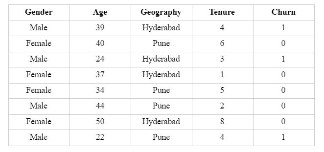
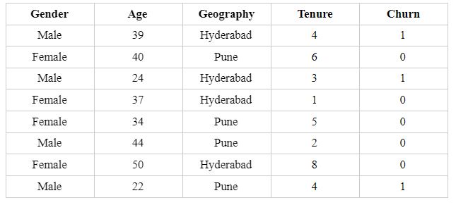
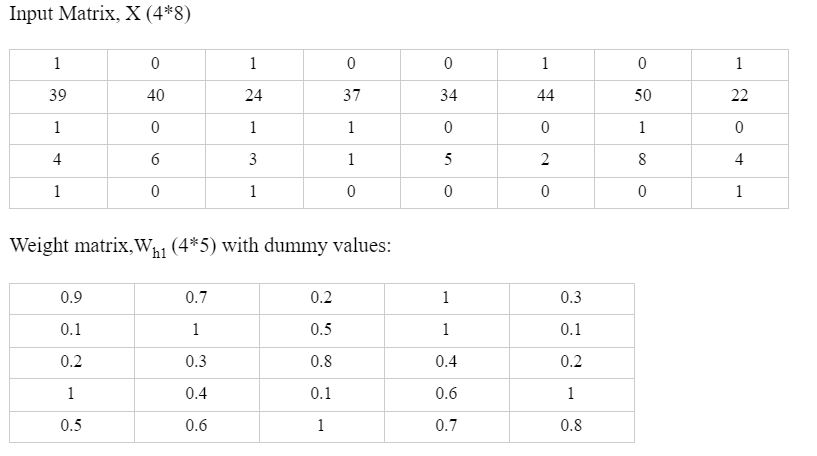
Let’s start with a binary classification problem where we want to classify whether the customer will churn or not churn. We will use a small dummy data for our understanding purpose with four input variables and eight observations.
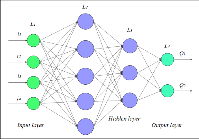
It has the following neural net with an architecture of [4, 5, 3, 2] and is depicted below:
For our purpose here, I will refer to the neurons in Hidden Layer L2 as N1, N2, N3, N4, N5 and N6, N7, N8 in the Hidden Layer L3, respectively in the linear order of their occurrence. In a classification problem, the output layer can either have one node or can have nodes equivalent to the number of the classes or the categories.
This network here is called Fully Connected Network (FNN) or Dense Network since every neuron has a connection with the node of the previous layer output. It is also known as the Feedforward Neural Network or Sequential Neural Network.
The equation for the neural network is a linear combination of the independent variables and their respective weights and bias (or the intercept) term for each neuron. The neural network equation looks like this:
Z = Bias + W1X1 + W2X2 + …+ WnXn
where,
There are three steps to perform in any neural network:
Firstly, we will understand how to calculate the output for a neural network and then will see the approaches that can help to converge to the optimum solution of the minimum error term.
The output layer nodes are dependent on their immediately preceding hidden layer L3, which is coming from the hidden layer 2 and those nodes are further derived from the input variables. These middle hidden layers create the features that the network automatically creates and we don’t have to explicitly derive those features. In this manner, the features are generated in Deep Learning models and this is what makes them stand out from Machine Learning.
So, to compute the output, we will have to calculate for all the nodes in the previous layers. Let us understand what is the mathematical explanation behind any kind of neural nets.
Now, as from the above architecture, we can see that each neuron cannot have the same general equation for the output as the above one. We will have one such equation per neuron both for the hidden and the output layer.
The nodes in the hidden layer L2 are dependent on the Xs present in the input layer therefore, the equation will be the following:
Similarly, the nodes in the hidden layer L3 are derived from the neurons in the previous hidden layer L2, hence their respective equations will be:
The output layer nodes are coming from the hidden layer L3 which makes the equations as:
Now, how many weights or betas will be needed to estimate to reach the output? On counting all the weights Wis in the above equation will get 51. However, no real model will have only three input variables to start with!
Additionally, the neurons and the hidden layers themselves are the tuning parameters so in that case, how will we know how many weights to estimate to calculate the output? Is there an efficient way than the manual counting approach to know the number of weights needed? The weights here are referred to the beta coefficients of the input variables along with the bias term as well (and the same will be followed in the rest of the article).
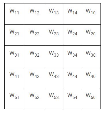
The structure of the network is 4,5,3,2. The number of weights for the hidden layer L2 would be determined as = (4 + 1) * 5 = 25, where 5 is the number of neurons in L2 and there are 4 input variables in L1. Each of the input Xs will have a bias term which makes it 5 bias terms, which we can also say as (4 + 1) = 5.
Therefore, the number of weights for a particular layer is computed by taking the product of (number of nodes/variables + bias term of each node) of the previous layer and the number of neurons in the next layer
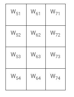
Similarly, the number of weight for the hidden layer L3 = (5 + 1) * 3 = 18 weights, and for the output layer the number of weights = (3 + 1) * 2 = 8.
The total number of weights for this neural network is the sum of the weights from each of the individual layers which is = 25 + 18 + 8 = 51
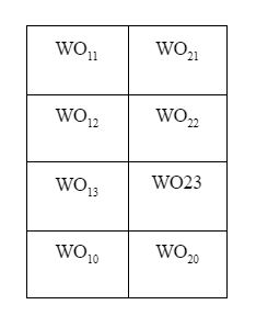
We now know how many weights will we have in each layer and these weights from the above neuron equations can be represented in the matrix form as well. Each of the weights of the layers will take the following form:
Hidden Layer L2 will have a 5 * 5 matrix as seen the number of weights is (4 + 1) * 5:
A 3*6 matrix for the hidden layer L3 having the number of weights as (5 + 1) * 3 = 18
Lastly, the output layer would be 4*2 matrix with (3 + 1) * 2 number of weights:
Okay, so now we know how many weights we need to compute for the output but then how do we calculate the weights? In the first iteration, we assign randomized values between 0 and 1 to the weights. In the following iterations, these weights are adjusted to converge at the optimal minimized error term.
We are so persistent about minimizing the error because the error tells how much our model deviates from the actual observed values. Therefore, to improve the predictions, we constantly update the weights so that loss or error is minimized.
This adjustment of weights is also called the correction of the weights. There are two methods: Forward Propagation and Backward Propagation to correct the betas or the weights to reach the convergence. We will go into the depth of each of these techniques; however, before that lets’ close the loop of what the neural net does after estimating the betas.
The next step on the ladder of computation of output is to apply a transformation on these linear equations. As we have a neural net related to classification at hand, how will this linear equation be applied in the cases when the output is to be categorized in classes?
For a binary classification problem, we know that Sigmoid is needed to transform the linear equation to a nonlinear equation. In case you are not sure why we use Sigmoid to transform a linear equation to a nonlinear equation, then would suggest refreshing the logistic regression.
For a particular node, the transformation is as follows:
N1 = W11*X1 + W12*X2 + W13*X3 + W14*X4 + W10
After implementing the Sigmoid transformation, it becomes:
h1 = sigmoid(N1)
where,
sigmoid(N1) = exp(W11*X1 + W12*X2 + W13*X3 + W14*X4 + W10)/(1+ exp(W11*X1 + W12*X2 + W13*X3 + W14*X4 + W10))
This alteration is applied on the hidden layers and the output layers and is known as the Activation or the Squashing Function. The transformation is required to bring non-linearity to the network as every business problem may not be solved linearly.
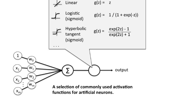
There are various types of activation functions available and each function has a different utilization. On the output layer, the activation function is dependent on the type of business problem. The squashing function for the output layer for binary classification is the Sigmoid. To know more about these functions and their applicability can refer to these blogs here and here.
Hence, to find the output we estimate the weights and perform the mathematical transformation. The output of a node is the outcome of this activation function.
Till this point, we have just completed step 1 of the neural network that is taking the input variables and finding the output. Then we calculate the error term. And mind you, right now this is only done for one record! We perform this entire cycle all over again for all the records!
Relax, we don’t have to do this manually. This is just the process, the network does these steps in its background. The idea here is to know how the network works, we don’t have to do it manually.
In the neural network, we can move from left to right and right to left as well. The right to left process of adjusting the weights from the Output to the Input layer is Backward Propagation (I will cover this in the next article).
The process of going from left to right i.e from the Input layer to the Output Layer is Forward Propagation. We move from left to right to adjust or correct the weights. We will understand how this mathematically works and update the weights to have the minimized loss function.
Our binary classification dataset had input X as 4 * 8 matrix with 4 input variables and 8 records and the Y variable is 2 * 8 matrix with two columns, for class 1 and 0, respectively with 8 records. It had some categorical variables post converting it to dummy variables, we have the set as below:
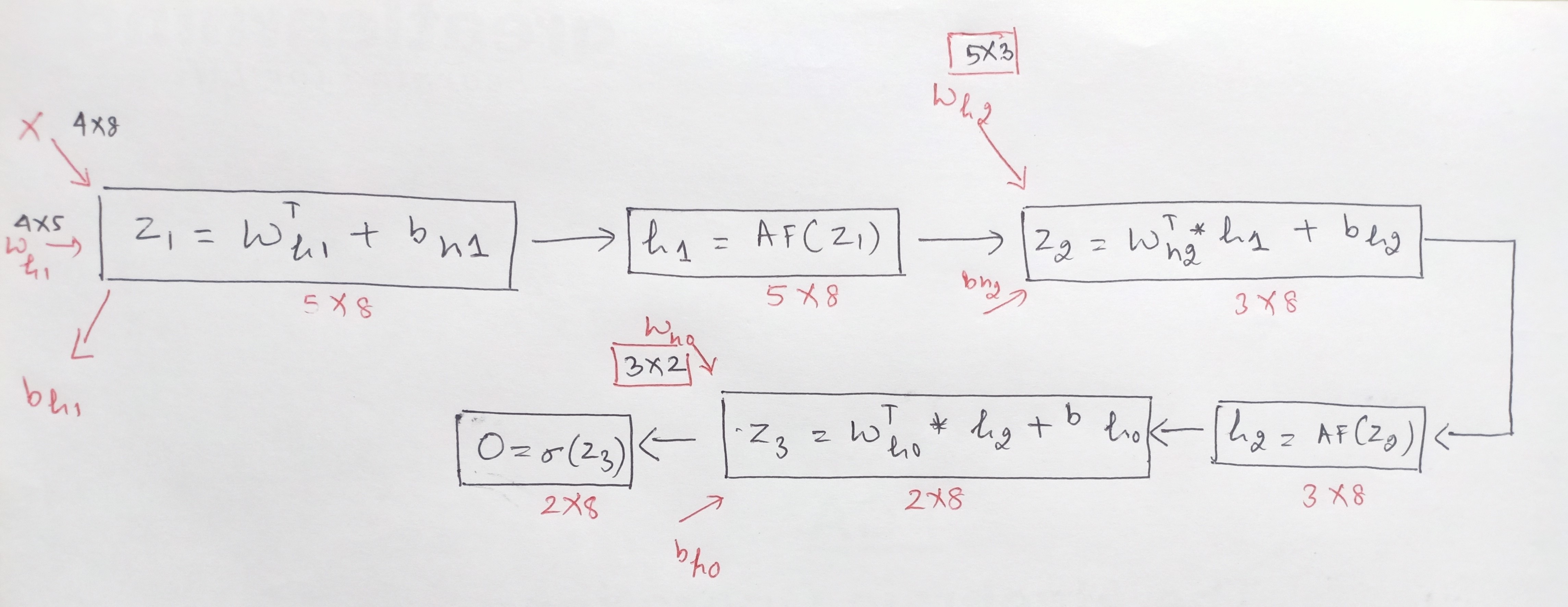
The idea here is that we start with the input layer of the 4*8 matrix and want to get the output of (2*8). The hidden layers and the neurons in each of the hidden layers are hyperparameters and so are defined by the user. How we achieve the output is via matrix multiplication between the input variables and the weights of each layer.
We have seen above that the weights will have a matrix for each of the respective layers. We perform matrix multiplication starting from the input matrix of 4 * 8 with the weight matrix between the L1 and L2 layer to get the next matrix of the next layer L3. Similarly, we will do this for each layer and repeat the process until we reach the output layer of the dimensions 2 * 8.
Please note the above explanation of the estimation of neurons was for a single observation, the network performs the entire above process for all the observations.
Now, let’s break down the steps to understand how the matrix multiplication in Forward propagation works:
We can multiply element by element but that result will be only for one observation or one record. To get the result for all the 8 observations in one go, we need to multiply the two matrices.
For matrix multiplication, the number of columns of the first matrix must be equal to the number of rows of the second matrix. Our first matrix of input has 8 columns and the second matrix of weights has 4 rows hence, we can’t multiply the two matrices.
So, what do we do? We take the transpose of one of the matrices to conduct the multiplication. Transposing the weight matrix to 5 * 4 will help us resolve this issue.
So, now after adding the bias term, the result between the input layer and the hidden layer L2, becomes Z1 = Wh1T * X + bh1.
5. The next step is to apply the activation function on Z1. Note, the shape of Z1 does not change by applying the activation function so h1 = activation function(Z1) is of shape 5*8.
6. In a similar manner to the above five steps, the network using the forward propagation gets the outcome of each layer:
Note that for the next layer between L2 and L3, the input this time will not be X but will be h1, which results from L1 and L2.
Z2 = Wh2T * h1 + bh2,
where ,
So, Z2 = Wh2T * h1 + bh2 with its matrix multiplication is:
Z2 = [(3*5) * (5*8)] + bh2 will result Z2 with dimension of 3*8 and post this again apply the activation function, which results in: h2 = activation function(Z2) is of shape 3*8.
7. We repeat these steps for the computation of the last layer.
This time for the next layer between L3 and L4, the input will be h2, resulting from L2 and L3.
Z3 = Wh0T * h2 + bh0,
So, Z3 = Wh0T * h2 + bh0, with its matrix multiplication is:
Z3 = [(2*3) * (3*8)] + bh0 will result in Z3 with the dimension of 2*8 and post this again apply the activation function, this time use Sigmoid to transform as need to get the output, which results in O = Sigmoid(Z3) is of shape 2*8.
After estimating the output using Forward propagation, then we calculate the error using this output, and this process of finding the weights to minimize the error continues until the optimal solution is achieved.
The other method and the preferred method to correct the weights is Backward Propagation which we shall explore in the next article.
A. The cost formula in a neural network, also known as the loss or objective function, measures the difference between predicted outputs and actual target values during training. It quantifies the network’s performance and aids in adjusting the model’s parameters to minimize errors. Common examples include mean squared error for regression tasks and cross-entropy for classification tasks.
A. The formula for deep network calculation involves sequentially computing the output of each layer. It starts with input data fed into the first layer, then successively applies activation functions to the weighted sum of inputs at each layer. This process continues until the output layer is reached, providing the final prediction or result of the deep neural network’s computation.
In conclusion, the estimation of neurons and forward propagation are fundamental concepts in neural networks. Estimating the number of neurons required in a neural network is crucial to avoid overfitting and underfitting, which can negatively impact the network’s performance. Forward propagation is the process of moving data through the neural network, allowing it to make predictions. This article has only touched the surface of these concepts, and there is much more to explore in the field of neural networks.
If you’re interested in learning more about neural networks and their applications, consider enrolling in our Blackbelt program. You can gain the skills and knowledge necessary to build and deploy neural networks and other advanced AI models. So, what are you waiting for? Join Blackbelt today and start your journey to becoming a data expert!
The media shown in this article are not owned by Analytics Vidhya and is used at the Author’s discretion.
Hi there! I am Neha Seth. I work as a Data Scientist in Larsen & Toubro Infotech (LTI). I hold a Postgraduate Program in Data Science & Engineering from the Great Lakes Institute of Management and a Bachelors in Statistics. I have been featured as Top 10 Most Popular Guest Authors in 2020 on Analytics Vidhya (AV). My area of interest lies in NLP and Deep Learning. I have also passed the CFA Program. You can reach out to me on LinkedIn and can read my other blogs for AV.
Lorem ipsum dolor sit amet, consectetur adipiscing elit,


Going great 👍
This article is helpful to understand how the nodes are estimated, how a neural network operates, its parameters, and the working of the forward propagation method. Nice
A lot of thanks, Neha Seth! This article is written in a very clear and fluent language. I wish you further development in your creativity.