Data analysis involves various techniques such as univariate analysis, which is the analysis of a single variable, as well as multivariate analysis, which is the analysis of multiple variables simultaneously. Data is everywhere around us, in spreadsheets, on various social media platforms, in survey forms, and more. The process of cleaning, transforming, interpreting, analyzing, and visualizing this data to extract useful information and gain valuable insights to make more effective business decisions is called Data Analysis.
Data Analysis can be organized into 6 types
- Exploratory Analysis
- Descriptive Analysis
- Inferential Analysis
- Predictive Analysis
- Causal Analysis
- Mechanistic Analysis
Here, we will dive deep into Exploratory Analysis,
This article was published as a part of the Data Science Blogathon.
Table of contents
Exploratory Analysis
The preliminary analysis of data to discover relationships between measures in the data and to gain an insight on the trends, patterns, and relationships among various entities present in the data set with the help of statistics and visualization tools is called Exploratory Data Analysis (EDA).
Exploratory data analysis is cross-classified in two different ways where each method is either graphical or non-graphical. And then, each method is either univariate, bivariate or multivariate.
Univariate Analysis
Uni means one and variate means variable, so in univariate analysis, there is only one dependable variable. The objective of univariate analysis is to derive the data, define and summarize it, and analyze the pattern present in it. In a dataset, it explores each variable separately. It is possible for two kinds of variables- Categorical and Numerical.
Some patterns that univariate analysis can easily identify include Central Tendency (mean, mode, and median), Dispersion (range, variance), Quartiles (interquartile range), and Standard Deviation.
Univariate data can be described through:
Frequency Distribution Tables
The frequency distribution table reflects how often an occurrence has taken place in the data. It gives a brief idea of the data and makes it easier to find patterns.
Example:
The list of IQ scores is: 118, 139, 124, 125, 127, 128, 129, 130, 130, 133, 136, 138, 141, 142, 149, 130, 154.
| IQ Range | Number |
| 118-125 | 3 |
| 126-133 | 7 |
| 134-141 | 4 |
| 142-149 | 2 |
| 150-157 | 1 |
Bar Charts
The bar graph is very convenient while comparing categories of data or different groups of data. It helps to track changes over time. It is best for visualizing discrete data.
#Adjust the output window size for better view
import matplotlib.pyplot as plt
fig = plt.figure()
ax = fig.add_axes([0,0,1,1])
courses = ['Machine Lerning','Web Development','App Development']
students_enrolled = [50,37,42]
ax.bar(courses,students_enrolled)
plt.show()
Histograms
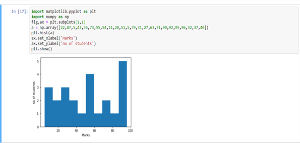
Histograms are similar to bar charts and display the same categorical variables against the category of data. Histograms display these categories as bins which indicate the number of data points in a range. It is best for visualizing continuous data.
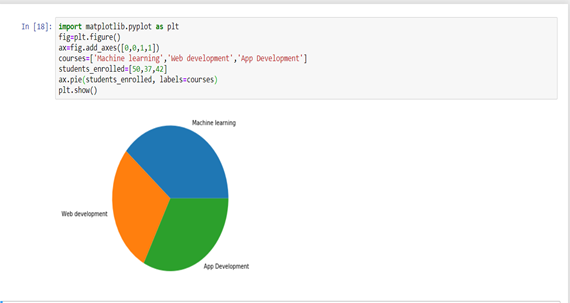
Pie Charts
Pie charts are mainly used to comprehend how a group is broken down into smaller pieces. The whole pie represents 100 percent, and the slices denote the relative size of that particular category.
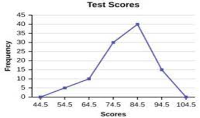
Frequency Polygons
Similar to histograms, you can use a frequency polygon to compare datasets or display the cumulative frequency distribution.
Bivariate Analysis
Bi means two and variate means variable, so here there are two variables. The analysis is related to cause and the relationship between the two variables. There are three types of bivariate analysis.
Bivariate Analysis of two Numerical Variables (Numerical-Numerical)
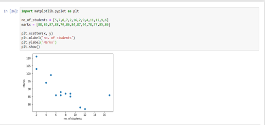
Scatter Plot
A scatter plot represents individual pieces of data using dots. These plots make it easier to see if two variables are related to each other. The resulting pattern indicates the type (linear or non-linear) and strength of the relationship between two variables.
Linear Correlation
Linear Correlation represents the strength of a linear relationship between two numerical variables. If there is no correlation between the two variables, there is no tendency to change along with the values of the second quantity.
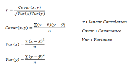
Here, r measures the strength of a linear relationship and is always between -1 and 1 where -1 denotes perfect negative linear correlation and +1 denotes perfect positive linear correlation and zero denotes no linear correlation.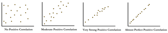
Bivariate Analysis of two categorical Variables (Categorical-Categorical)
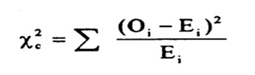
Chi-square Test
The chi-square test determines the association between categorical variables. Analysts calculate it based on the difference between expected frequencies and observed frequencies in one or more categories of the frequency table. A probability of zero indicates a complete dependency between two categorical variables and a probability of one indicates that two categorical variables are completely independent.
Here, subscript c indicates the degrees of freedom, O indicates observed value, and E indicates expected value.
Bivariate Analysis of one numerical and one categorical variable (Numerical-Categorical)
Z-test and t-test
Z and T-tests are important to calculate if the difference between a sample and population is substantial.
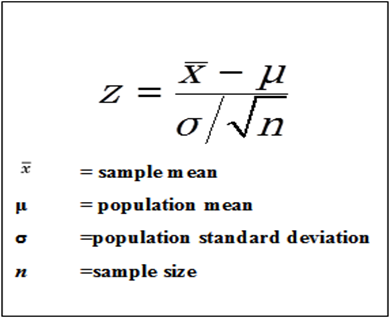
If the probability of Z is small, the difference between the two averages is more significant.
T-Test
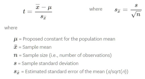
If the sample size is large enough, then we use a Z-test, and for a small sample size, we use a T-test.
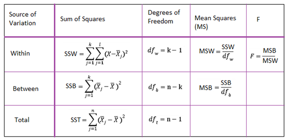
ANALYSIS OF VARIANCE (ANOVA)
The ANOVA test is used to determine whether there is a significant difference among the averages of more than two groups that are statistically different from each other. This analysis is appropriate for comparing the averages of a numerical variable for more than two categories of a categorical variable.
Multivariate Analysis
Multivariate analysis becomes necessary when analysts need to examine more than two variables simultaneously. Visualizing relationships among four variables in a graph presents a tremendous challenge for the human brain, so analysts use multivariate analysis to study more complex data sets. Types of Multivariate Analysis include Cluster Analysis, Factor Analysis, Multiple Regression Analysis, Principal Component Analysis, etc. More than 20 different ways to perform multivariate analysis exist and which one to choose depends upon the type of data and the end goal to achieve. The most common ways are:
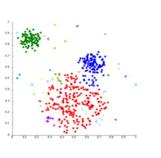
Cluster Analysis
Cluster Analysis classifies different objects into clusters in a way that the similarity between two objects from the same group is maximum and minimal otherwise. It is used when rows and columns of the data table represent the same units and the measure represents distance or similarity.
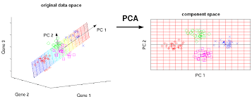
Principal Component Analysis (PCA)
Principal Components Analysis (PCA) reduces the dimensionality of a data table with a large number of interrelated measures. This process converts the original variables into a new set of variables known as the “Principal Components” of PCA.
PCA addresses datasets that exhibit multicollinearity. Although least squares estimates may show bias, the distance between variances and their actual values can be significantly large. So, PCA adds some bias and reduces standard error for the regression model.
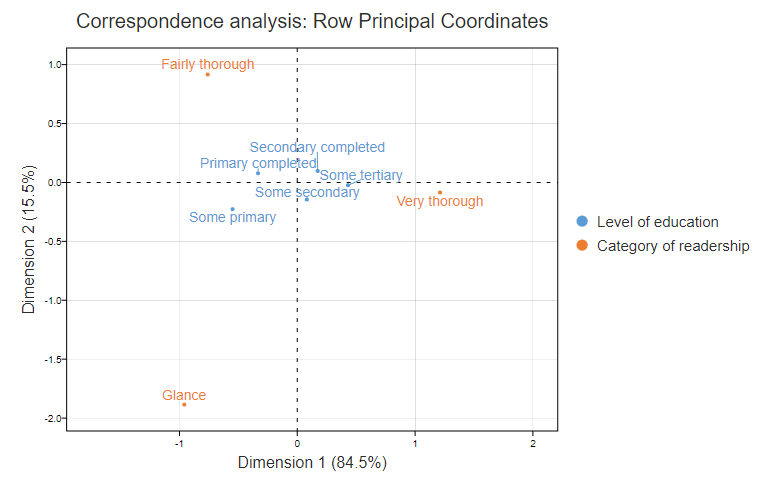
Correspondence Analysis
Correspondence Analysis using the data from a contingency table shows relative relationships between and among two different groups of variables. A contingency table is a 2D table with rows and columns as groups of variables.
Conclusion
We’ve explored various methods to understand data, from examining one thing at a time to analyzing how different factors relate. This helps uncover patterns and insights, aiding in better decision-making. Overall, the journey through different analyses equips us with valuable knowledge to inform future actions and research.
I hope you now have a better understanding of various techniques used in Univariate, Bivariate, and Multivariate Analysis.
Analytics Vidhya does not own the media shown in this article, and the author uses it at their discretion.
Frequently Asked Questions
Q1. What is exploratory analysis?
A. Exploratory analysis serves as a data analysis approach that aims to gain initial insights and understand patterns or relationships within the dataset.
Q2. What are univariate analysis techniques?
A. Univariate analysis involves analyzing one variable at a time to understand its distribution, central tendency, and variability.
Q3. What is bivariate analysis?
A. Bivariate analysis examines the relationship between two variables to understand how they interact or influence each other.
Q4. How does multivariate analysis differ from univariate and bivariate analysis?
A. Multivariate analysis involves analyzing multiple variables simultaneously to explore complex relationships and patterns within the data. It goes beyond examining individual or paired variables.


It was really useful, helping and knowledgeable enough in this generation. Thank you for your concern!