Estimators – An Introduction to Beginners in Data Science

This article was published as a part of the Data Science Blogathon.

Introduction

Not having much information about the distribution of a random variable can become a major problem for data scientists and statisticians. Consider, a researcher trying to understand the distribution of Choco-chips in a cookie (a very popular example of Poisson distribution). The researcher is well aware that the distribution of Choco-chips follows a Poisson distribution, but does not know how to estimate the parameter λ of the distribution.

A parameter is essentially a numerical characteristic of a distribution (or any statistical model in general). Normal distributions have µ & σ as parameters, uniform distributions have a & b as parameters, and binomial distributions have n & p as parameters. These numerical characteristics are vital for understanding the size, shape, spread, and other properties of a distribution. In the absence of the true value of the parameter, it seems that the researcher may not be able to continue her investigation. But that’s when estimators step in.

Estimators are functions of random variables that can help us find approximate values for these parameters. Think of these estimators like any other function, that takes an input, processes it, and renders an output. So, the process of estimation goes as follows:

1) From the distribution, we take a series of random samples.

2) We input these random samples into the estimator function.

3) The estimator function processes it and gives a set of outputs.

4) The expected value of that set is the approximate value of the parameter.

Example

Let’s take an example. Consider a random variable X showing a uniform distribution. The distribution of X can be represented as U[0, θ]. This has been plotted below:

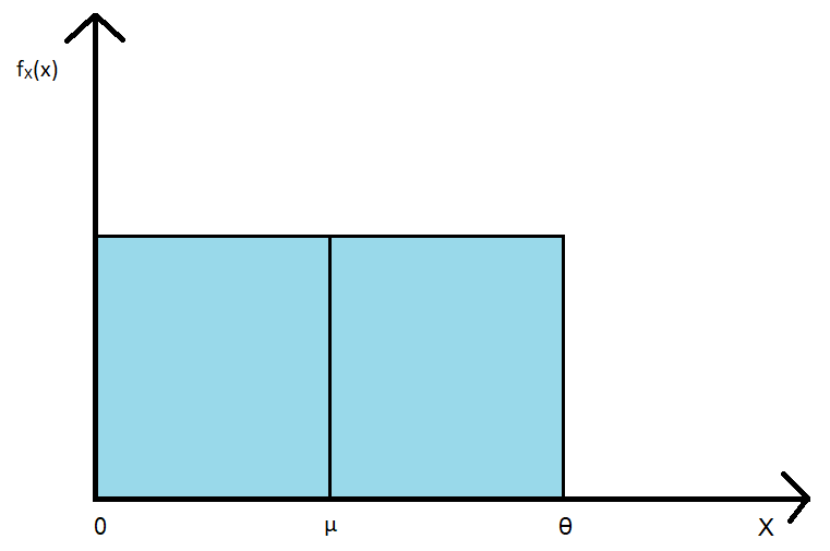
(Figure A)

We have the random variable X and its distribution. But we don’t know how to determine the value of θ. Let’s use estimators. There are many ways to approach this problem. I’ll discuss two of them:

1) Using Sample Mean

We know that for a U[a, b] distribution, the mean µ is given by the following equation:

For U[0, θ] distribution, a = 0 & b = θ, we get:

Thus, if we estimate µ, we can estimate θ. To estimate µ, we use a very popular estimator called the sample mean estimator. The sample mean is the sum of the random sample value drawn divided by the size of the sample. For instance, if we have a random sample S = {4, 7, 3, 2}, then the sample mean is (4+7+3+2)/4 = 4 (the average value). In general, the sample mean is defined using the following notation:

Here, µ-hat is the sample mean estimator & n is the size of the random sample that we take from the distribution. A variable with a hat on top of it is the general notation for an estimator. Since our unknown parameter θ is twice of µ, we arrive at the following estimator for θ:

We take a random sample, plug it into the above estimator, and get a number. We repeat this process and get a set of numbers. The following figure illustrates the process:

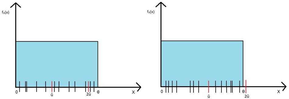
(Figure B)

The lines on the x-axes correspond to the values present in the sample taken from the distribution. The red lines in the middle indicate the average value of the sample, and the red lines at the end are twice that average value i.e., the expected value of θ for one sample. Many such samples are taken, and the estimated value of θ for each sample is noted. The expected value/mean of that set of numbers gives the final estimate for θ. It can be mathematically proved (using properties of expectation):

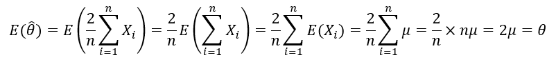
It is seen that the expectation of the estimator is equal to the true value of the parameter. This amazing property that certain estimators have is called unbiasedness, which is a very useful criterion for assessing estimators.

2) Maximum Value Method

This time, instead of using mean, we’ll use order statistics, particularly the nth order statistic. The nth order statistic is defined as the nth smallest value of a random sample of size n. In other words, it’s the maximum value of a random sample. For instance, if we have a random sample S = {4, 7, 3, 2}, then the nth order statistic is 7 (the largest value). The estimator is now defined as follows:

We follow the same procedure- take random samples, input them, collect the output and find the expectation. The following figure illustrates the process:

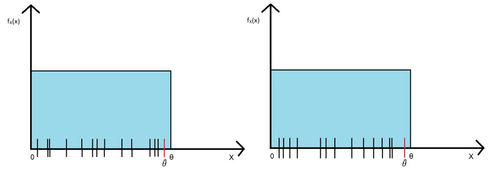
(Figure C)

As noted previously, the lines on the x-axes are the values present in one sample. The red lines at the end are the maximum value for that sample i.e., the nth order statistic. Two random samples are shown for reference. However, we need to take much larger samples. Why? To prove it, we’ll use the general expression for the PDF (Probability Distribution Function) of nth order statistics for U[a, b] distribution:

For U[0, θ] distribution, a = 0 & b = θ, we get:

Using the integral form of expectation of a continuous variable,

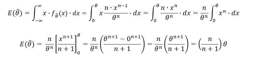
Unlike before, no exact equality has been ascertained between the expectation of θ-hat & θ. This is because the nth order statistic estimator is biased. We can observe this bias on comparing figures B & C. In figure B, both positive (θ-hat > θ) and negative (θ-hat < θ) deviations are possible with equal probability (as shown). These deviations can cancel each other out, making the sample mean estimator unbiased. However, in figure C, only negative deviations are possible. Why? Because the maximum value of a random sample will always be lesser than the range [0, θ] of the distribution. Consequently, negative bias steps in.

Does that mean that we cannot use this estimator? Certainly not. As discussed earlier, the estimator bias can be significantly lowered by taking large n. For large values of n, n = n+1 (approximately). Thus, we get:

The Bottom Line

Hence, we have successfully solved our problem through estimators. We also learned a very important property of estimators- unbiasedness. While this may have been an extensive read, it’s imperative to acknowledge that the study of estimators is not restricted to just the above-explained concepts. Various other properties of estimators such as their efficiency, robustness, mean squared error, and consistency are also vital to deepen our understanding of them.

The media shown in this article are not owned by Analytics Vidhya and is used at the Author’s discretion.