Image Classification with Tensorflow: Data Augmentation on Streaming Data (Part 2)

This article was published as a part of the Data Science Blogathon

Introduction

This article is in continuation with Part 1 where we discussed Data pipelines in general and how we can use TensorFlow Data Pipelines: Tensorflow Datasets. For a brief recall, we created a Binary Image classifier from Extracting, Transforming, and Loading the data from “TensorFlow Datasets” on the “Horses-and-Human” dataset. If you are unfamiliar with the concept, I would advise that you check out that article as well.

Here in this article, we will be creating a similar Binary Image classifier but unlike earlier, this time we will deal with overfitting and through Data Augmentation. We will be using Data augmentation as sequence model layers, these layers will transform the streaming data in the model before actually going into Convolutional and MaxPooling layers. This gives us the leverage of using the already stored data with the more diverse examples on the runtime model training. But before any of that:

What is Data Augmentation?

Data Augmentation is a very popular technique in image processing, especially computer vision to increase the diversity and amount of training data by applying random (but realistic) transformations. For example, Image resizes, Image rotation, Image flip, and many more. This technique helps us get a more diverse nature of already contained data resulting in a better training set and hence a better-trained model.

NOTE: In Deep Learning when we use Data Augmentation, we apply the technique only on training data not on validation data, nor on testing data.

I am skipping the code explanation of those parts that are already covered in Part 1 and head straight to this article’s content.

Let’s CODE:

Importing the libraries and using TensorFlow datasets for retrieving the data

import numpy as np
import matplotlib.pyplot as plt
import tensorflow as tf
import tensorflow_datasets as tfds
from tensorflow.keras import layers

train_dataset,info = tfds.load('horses_or_humans', with_info = True, split='train', as_supervised=True)
val_dataset,val_info = tfds.load("horses_or_humans", with_info=True, split='test', as_supervised=True)

tensorflow.data.Dataset Object that these data pipelines create is a Python iterator. So, let us look at one of the examples in the “train_dataset“

get_label_name = info.features["label"].int2str
image, label = next(iter(train_dataset))
_ = plt.imshow(image)
_ = plt.title(get_label_name(label))

 

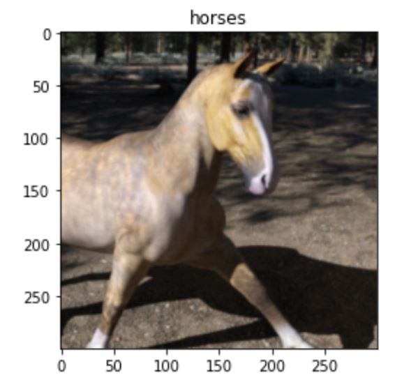
> get_label_name is a function that will change the label (0,1) into string (“horses”, “humans”)

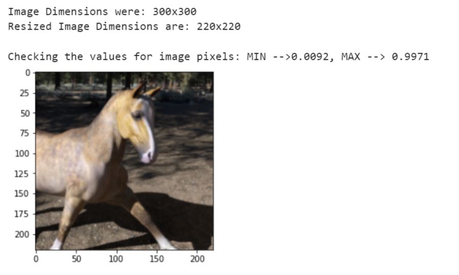
Let’s create our first sequence of data augmentation layers that includes Resizing and Rescaling. I personally call them light augmentation, as visually they look almost the same except for their changed shape and underlying pixel values. Here, our raw images in the dataset are 300 x 300 x 3 pixels. (3 at the end is for RGB channel in images, let’s ignore this in this article)

With Resizing: I am changing the dimension of the images : from 300 x 300 x 3 –> 220 x 220 x 3

With Rescaling: I am changing all the pixel values that originally lie between [0,255] –> [0,1], Image will look the same but the underlying pixel values will change, although relatively they represent the same colors and features.

IMG_SIZE = 220
## Becuase Pixel range in Images are between [0,255], To rescale an input in the [0, 255] range
# to be in the [0, 1] range, you would pass scale=1./255
resize_and_rescale = tf.keras.Sequential([
            layers.experimental.preprocessing.Resizing(IMG_SIZE, IMG_SIZE, input_shape=[300,300,3]),
            layers.experimental.preprocessing.Rescaling(1./255)
])

Let’s visualize and see the results.

result  = resize_and_rescale(image)
plt.imshow(result)
print("Image Dimensions were: {0}x{1}".format(image.shape[0], image.shape[1]))
print("Resized Image Dimensions are: {0}x{1}".format(result.shape[0], result.shape[1]))
print()
print(f"Checking the values for Resulted image pixels: MIN -->{result.numpy().min():.4f}, MAX --> {result.numpy().max():.4f}")

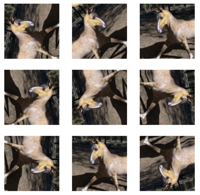
Moving forward to another set of augmentation layers, I call these heavy augmentations because the results from them change the visual of an image in some or the other sort. Look for yourself here.

NOTE: Remember all these layers work with 4 dimensions of inputs, 4th one is for the number of images in a batch i.e. BATCH_SIZE (It came first from every other value in the shape), for visual inspection we will use tf.expand_dims function to help in the matter.

## Heavier Augmentation
data_augmentation = tf.keras.Sequential([
                            layers.experimental.preprocessing.RandomFlip("horizontal_and_vertical"),
                            layers.experimental.preprocessing.RandomRotation((-0.2, 0.3))
])

With RandomFlip: I am Flipping the image randomly in either of the direction (horizontally or vertically)

With RandomRotation: I am rotation the images with a random degree chosen from the range provided in the functional argument (-0.2, 0.3) –> (-20 degrees to 30 degrees clockwise).

print(image.shape)
image = tf.expand_dims(image, 0)
print(image.shape)

Let’s Visualize how the randomize the effect in these 9 iterations.

plt.figure(figsize = (10,10))
for i in range(9):
  augmented_image = data_augmentation(image)
  ax = plt.subplot(3,3,i+1)
  plt.imshow(augmented_image[0])
  plt.axis("off")

 

Shuffling and Batching the train_dataset, and Batching the test_dataset as done earlier in Part 1.

train_dataset = train_dataset.shuffle(100).batch(8)
val_dataset = val_dataset.batch(8)

One thing that is really important to notice here, is the Batch size. I have reduced the batch size from 32 to 8 compared to Part 1’s code. I did it after hyperparameter tuning and experimentation with my model. My model was giving random result with validation dataset at training and hence a lot of noise in loss and accuracy, so to let the model not generalize too much on all the augmented data, I reduced the batch size to reduce the number of images used in every time step to calculate loss and optimize the parameters through gradients.

Let’s see how it’s very simple to accumulate all the layers created for augmentation with each and other and the main CNN model layers.

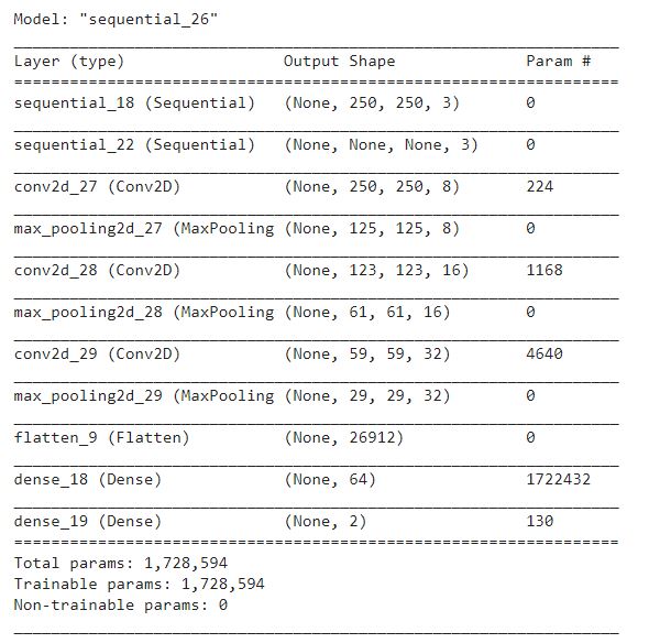
model = tf.keras.models.Sequential([
                                   resize_and_rescale,
                                   data_augmentation,
                                   tf.keras.layers.Conv2D(filters=8, kernel_size = 3, activation='relu', padding='same'),
                                   tf.keras.layers.MaxPooling2D(),
                                   tf.keras.layers.Conv2D(filters = 16, kernel_size = 3, activation = 'relu'),
                                   tf.keras.layers.MaxPooling2D(),
                                    tf.keras.layers.Conv2D(filters = 32, kernel_size = 3, activation = 'relu'),
                                   tf.keras.layers.MaxPooling2D(),
                                   tf.keras.layers.Flatten(),
                                   tf.keras.layers.Dense(units=64, activation = 'relu'),
                                   tf.keras.layers.Dense(units = 2, activation='softmax')
])
model.summary()

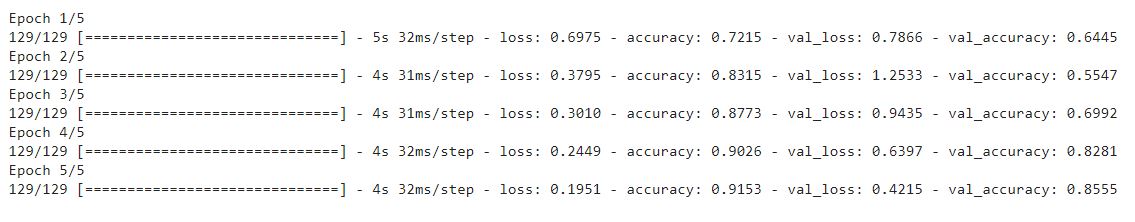
Now, we got really close to our final trained model, the only things left to do is compile the model and fit it on the training dataset and validate the training through the validation dataset. During compilation, I wanted the freedom to change my learning rate for hyperparameter tuning so, I used RMSprop directly from tensorflow.keras.optimizers

In just 5 epochs compared to 8 earlier, look at the result and convergence of loss and accuracy of both training data and validation data.

from tensorflow.keras.optimizers import RMSprop
model.compile(loss="sparse_categorical_crossentropy", optimizer=RMSprop(learning_rate=0.001), metrics=['accuracy'])
history = model.fit(train_dataset, epochs=5, validation_data=val_dataset)

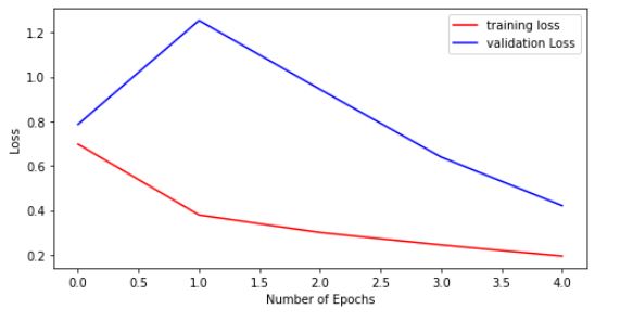
At last, Visualize the training and validation loss and accuracy through some plots.

## Loss Plot

plt.figure(figsize=(8, 4))
plt.plot(range(5), history.history['loss'], 'r', label='training loss')
plt.plot(range(5), history.history['val_loss'], 'b', label='validation Loss')
plt.legend()
plt.xlabel('Number of Epochs')
plt.ylabel("Loss")
plt.show()

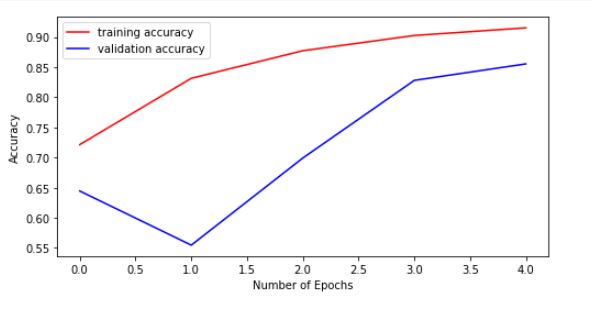
## Accuracy Plot

plt.figure(figsize=(8, 4))
plt.plot(range(5), history.history['accuracy'], 'r', label='training accuracy')
plt.plot(range(5), history.history['val_accuracy'], 'b', label='validation accuracy')
plt.legend()
plt.xlabel('Number of Epochs')
plt.ylabel("Accuracy")
plt.show()

 

Well, this was the end of this series of Binary Image Classification on Horses and Humans dataset with Tensorflow and their data pipelines (Tensorflow datasets) trained with some Data augmentation involved to avoid overfitting on the data.

Gargeya Sharma

B.Tech Computer Science 3rd year

Specialized in Data Science and Deep Learning

Data Scientist Intern at Upswing Cognitive Hospitality Solutions

For more info check out my Github Home Page

The media shown in this article are not owned by Analytics Vidhya and is used at the Author’s discretion.

Gargeya Sharma 06 Jul 2021