Simplifying Maths behind Principal Component Analysis
This article was published as a part of the Data Science Blogathon
PCA is the most important technique for dimensionality reduction for linear datasets. It is a nonparametric and simple method yet produces powerful results.
Do you know how PCA works with such ease and makes life simple for us?
In my previous article, I explained the working of PCA (without mathematics) along with Python implementation. Here, we will discuss the basic mathematical part of PCA with python implementation from scratch.
We need to learn few terms below before we start the discussion about PCA.
Covariance: Covariance is used to depict the relationship between two variables. If the covariance is positive then two variables tend to move in the same direction and if the covariance is negative then two variables tend to move in the opposite direction. In case covariance is 0 then we can state that there exists no relationship between two attributes.
Variance: It is the spread of the data. It tells us how far the values are from the mean.
We can summarize the basic steps of PCA as below. We will figure out these steps in detail.
- Standardization of data
- Computation of Covariance Matrix
- Calculation of Eigenvector and Eigenvalue
- Selection of number of Principal Components
- Multiplication of principal components with original data to create the newly transformed data set.
Let us take a simple data example. Assume we have two variables: “Salary” and “Expense
##Creating a dummy dataset
import pandas as pd
import numpy as np
import matplotlib.pyplot as plt
data = np.array([[1000 ,500],[2000, 800],[3000 ,1100],[4000 ,1500],[5000 ,1800],[8000,1900]])
df = pd.DataFrame(data,columns = ['Salary','Expense'])
##Scatterplot to check the spread and visualize the correlation
import seaborn as sns
plot = sns.lmplot(x='Salary', y='Expense', data=df, ci=None)
plt.title("Salary vs Expense")
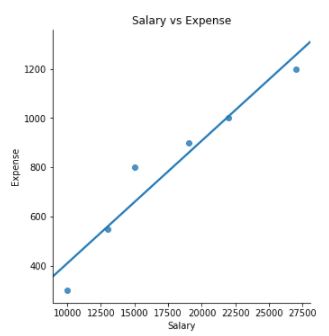
Now we will see how the covariance matrix will look like for the above two attributes.
![]()
![]()
Since we have two attributes in our data i.e. salary and expense; hence covariance matrix will be of shape 2×2. Please observe the below formula for covariance and variance. If x and y are the same then it will yield variance for the same attribute. Therefore, in the above covariance matrix, diagonal elements will yield variance for salary and expense. Also, one of the property of covariance is that it is symmetric i.e. covariance(x,y) = covariance(y,x) which tells us that covariance(salary, expense) = covariance(expense, salary)
Before we move further we need to know about eigenvectors and eigenvalues.
Eigenvectors and Eigenvalues: Magicians behind PCA
These terms sound quite complex but not that difficult to understand. These terms play the most important role in PCA.
Eigenvector is a non-zero vector that only changes the magnitude not direction when subjected to a linear transformation.
It means that if we multiply a non-zero vector with the above covariance matrix then the result would be a scaled version of the initial vector and that scaled value is the eigenvalue.
Mathematically, when an eigenvector is multiplied with a vector will give the product of the eigenvector and a scalar value.
![]()
Here A is any matrix, v is eigenvector and lambda is the eigenvalue.
In the below graph; Two vectors v and w when multiplied with a matrix A behave differently.
v becomes Av but still has the same direction (i.e. it has been scaled by A without change in its span). On the other hand, w becomes Aw, and the direction of w and Aw is different as well. Here we can conclude that v is an eigenvector and w is not an eigenvector.
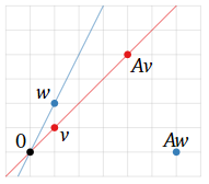
The above graph is taken from https://textbooks.math.gatech.edu/ila/eigenvectors.html
Once we have computed eigenvalues and eigenvectors for our covariance matrix we need to sort them in the decreasing order of the eigenvalue. These eigenvalues represent the variance of the data. We know that we will have the same number of principal components as we have attributes in data because these components are linear combinations of input data. Now we will select the first k components i.e. first k eigenvectors with the highest eigenvalues.
Important point to note is that principal components are uncorrelated as they are orthogonal to each other i.e. they are perpendicular to each other
Now we will continue the Python implementation of dummy data and standardize our data.
###Standardization of data which is essential for PCA
import warnings
warnings.filterwarnings('ignore')
from sklearn.preprocessing import StandardScaler
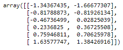
ss = StandardScaler()
scaled = ss.fit_transform(data)
scaled
###Compute covariance matrix and calculation of eigenvalue and eigenvectors
from numpy import linalg
cov = np.cov(scaled[:,0], scaled[:,1])
val, vec = linalg.eig(cov)
print("Below we have eigenvectors from the covariance matrix")
print(vec)
print("n Eigen Values for corresponding eigenvector")
print(val)
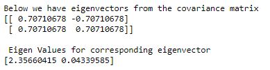
Now we have eigenvalues and corresponding eigenvectors. Different columns of the eigenvector matrix depicts different eigenvectors. We will choose an eigenvector corresponding to the highest eigenvalue and that is our first principal component.
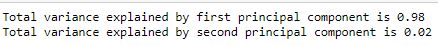
In case we have a large number of eigenvectors and eigenvalues; we will sort the eigenvalues in decreasing order of explained variance and then we will select the desirable number of components. Here first principal component is explaining 98% variance hence we will select the first component.
##Variance explained by each component
var_exp_1 = print('Total variance explained by first principal component is',round(val[0]/val.sum(),2))
var_exp_2 = print('Total variance explained by second principal component is',round(val[1]/val.sum(),2))
When we select the number of eigenvectors (having large eigenvalue) and form a matrix of those vectors then it is called feature vector.
Important point to note here is that if we choose k eigenvectors out of n then we have moved first step towards dimensionality reduction as dateset is reduced to k features now.
Let us take an example of our python output. We achieved the below feature vector corresponding to the highest eigenvalue.
array([0.70710678, 0.70710678])
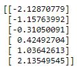
Now with the help of the above feature vector, we will project the data from the original axes into principal component axes. We will multiply the feature vector with original standardized data and obtain new transformed features.
#multiply the original data with the eigen vector
final_data = np.dot(scaled, np.array(vec.T[0]))
print(final_data)
To verify the results obtained from the manual process, the below calculation was done using sklearn PCA
from sklearn.decomposition import PCA
pca = PCA(n_components=1)
pca.fit(scaled)
print("Varaince explained by principal component is n", pca.explained_variance_ratio_)
print("Final output after PCA n",pca.transform(scaled)[:,0])
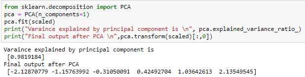
We can see here that our data which was having 2-Dimensions now can be projected in 1-Dimension space and that too while retaining 98% of the information.
I hope you found this article helpful 🙂
References:
https://textbooks.math.gatech.edu/ila/eigenvectors.html
https://strata.uga.edu/software/pdf/pcaTutorial.pdf
The media shown in this article are not owned by Analytics Vidhya and is used at the Author’s discretion.


