Image Denoising using AutoEncoders -A Beginner’s Guide to Deep Learning Project

This article was published as a part of the Data Science Blogathon

Introduction

Let’s start our discussion with understanding the meaning of the term “Image Denoising” which is also our article title –

Image Denoising is the process of removing noise from the Images

The noise present in the images may be caused by various intrinsic or extrinsic conditions which are practically hard to deal with. The problem of Image Denoising is a very fundamental challenge in the domain of Image processing and Computer vision. Therefore, it plays an important role in a wide variety of domains where getting the original image is really important for robust performance.

Let’s see how a noisy image looks like:

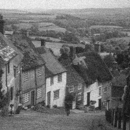
An example of Image with Noise

                                              Image Source: Link

So, In this article, we will see how we can remove the noise from the noisy images using autoencoders or encoder-decoder networks. In this article, I will implement the autoencoder using a Deep Artificial neural network. Probably, in my next article, I will also describe the autoencoder using a Deep Convolutional Neural network for the same problem statement. So, try this and stay tuned with us for my next tutorial.

Now, let’s also see that how the images look after removing the noise:

Before and After the Noise Removal of an Image of a Playful Dog

                                                     Image Source: Link

Now before doing any further delay, let’s start our discussion by revising some of the basic concepts about autoencoders.

Overview of Encoder-Decoder Network (Autoencoders) 

Autoencoder is an unsupervised artificial neural network that is trained to copy its input to output. In the case of image data, the autoencoder will first encode the image into a lower-dimensional representation, then decodes that representation back to the image. Encoder-Decoder automatically consists of the following two structures:

• The encoder- This network downsamples the data into lower dimensions.
• The decoder- This network reconstructs the original data from the lower dimension representation.

The lower dimension (i.e, output of encoder network) representation is usually known as latent space representation.

The one thing which we must remember about autoencoders is that they are only able to compress the data that is similar to what they have been trained on. They are also lossy in nature which means that the output will be degraded with respect to the original input.

They are trained similarly to Artificial Neural Networks via backpropagation.

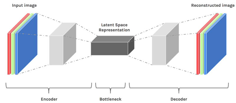
Figure Showing the architecture of an Encoder-Decoder (Autoencoder) Network

                                                             Image Source: Link

Let’s start our implementation! 😊

Load the necessary Libraries

The first step is to load the necessary Python libraries. We will import libraries such as numpy for optimizing the matrix multiplications, matplotlib for data visualization purposes such as plotting the images, Sequential model from Keras gives us an empty box in which we are adding several dense (i.e, fully connected) layers according to our architecture, Dense to create the fully connected layers in our network, MNIST to import the dataset from Keras directly.

import numpy 
import matplotlib.pyplot as plt
from keras.models import Sequential
from keras.layers import Dense
from keras.datasets import mnist

Now, we completed our first step of importing the necessary libraries, let’s go ahead and load the dataset in the form of numpy.

Load Dataset in Numpy Format

In this article, we will be using the MNIST dataset, which is a simple computer vision dataset. It consists of images of handwritten digits in the form of a greyscale. It also includes labels for each image, telling us which digit it is (i.e, output for each image). It means we have a labelled data in our hands to work with. Each image in the MNIST dataset is 28 pixels by 28 pixels.

Let’s see some of the images from the MNIST dataset:

We will split our MNIST data into two parts:

• Training Dataset: 60,000 data points belong to the training dataset, and
• Testing Dataset: 10,000 data points belongs to the test dataset.

(X_train, y_train), (X_test, y_test) = mnist.load_data()

Output:

Let’s take a look at the shape of our NumPy arrays with the help of the following lines of codes:

X_train.shape

Output:

(60000, 28, 28)

The above output indicates that we have 60,000 training images and each consists of 28 by 28 pixels.

X_test.shape

Output:

(10000, 28, 28)

The above output indicates that we have 10,000 testing images and each consists of 28 by 28 pixels.

Plot Images as a Grey Scale Image

Now, upto the above sections, we will load the complete dataset, and also divide it into training and testing sets. So, in this section, we will plot some of the images from our dataset using the matplotlib library, and specifically, we are using the subplot function of the matplotlib library to plot more than one image simultaneously.

plt.subplot(221)
plt.imshow(X_train[0], cmap=plt.get_cmap('gray'))
plt.subplot(222)
plt.imshow(X_train[1], cmap=plt.get_cmap('gray'))
plt.subplot(223)
plt.imshow(X_train[2], cmap=plt.get_cmap('gray'))
plt.subplot(224)
plt.imshow(X_train[3], cmap=plt.get_cmap('gray'))
# show the plot
plt.show()

Output:

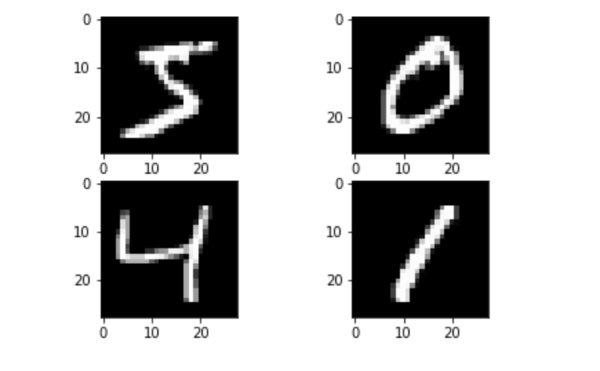
Image Source: Author

Formatting Data for Keras

We can flatten the 2-D array of images into a vector of 28×28=784 numbers. It is irrespective of how we flatten the array, as long as we’re consistent between images. From this perspective, the MNIST images are just a bunch of points in a vector space of 784-dimensional. But the data should always be of the format “(Number of data points, data point dimension)”. In this case, the training data will be of format 60,000×784.

num_pixels = X_train.shape[1] * X_train.shape[2]
X_train = X_train.reshape(X_train.shape[0], num_pixels).astype('float32')
X_test = X_test.reshape(X_test.shape[0], num_pixels).astype('float32')
X_train = X_train / 255
X_test = X_test / 255

Let’s again take a look at the shape of our NumPy arrays with the help of the following lines of codes:

X_train.shape

Output:

(60000, 784)

X_test.shape

Output:

(10000, 784)

Adding Noise to Images

While solving the problem statement, we have to remember our goal which is to make a model that is capable of performing noise removal on images. To be able to do this, we will use existing images and add them to random noise. Here we will feed the original images as input and we get the noisy images as output and our model (i.e, autoencoder) will learn the relationship between a clean image and a noisy image and learn how to clean a noisy image. So let’s create a noisy version of our MNIST dataset and give it as input to the decoder network.

We start with defining a noise factor which is a hyperparameter. The noise factor is multiplied with a random matrix that has a mean of 0.0 and a standard deviation of 1.0. This matrix will draw samples from a normal (Gaussian) distribution. While adding the noise, we have to remember that the shape of the random normal array will be similar to the shape of the data you will be adding the noise.

noise_factor = 0.2
x_train_noisy = X_train + noise_factor * numpy.random.normal(loc=0.0, scale=1.0, size=X_train.shape)
x_test_noisy = X_test + noise_factor * numpy.random.normal(loc=0.0, scale=1.0, size=X_test.shape)
x_train_noisy = numpy.clip(x_train_noisy, 0., 1.)
x_test_noisy = numpy.clip(x_test_noisy, 0., 1.)

After seeing the above code, you might think that why does this clip function is used here?

To ensure that our final images array item values are within the range of 0 to 1, we may use np.clip method. The clip is a Numpy function that clips the values outside of the Min-Max range and replaces them with the designated min or max value.

Let’s see how the noisy images look like:

Noisy Images of Handwritten Digits

Defining an Encoder-Decoder network

It will have an input layer of 784 neurons since we have an image size of 784 due to 28 by 28 pixels present (i.e. we have the input dimension and an output layer of 784 neurons).

# create model
model = Sequential()
model.add(Dense(500, input_dim=num_pixels, activation='relu'))
model.add(Dense(300, activation='relu'))
model.add(Dense(100, activation='relu'))
model.add(Dense(300, activation='relu'))
model.add(Dense(500, activation='relu'))
model.add(Dense(784, activation='sigmoid'))

Compiling the model

Once the model is defined, we have to compile it. While compiling we provide the loss function to be used, the optimizer, and any metric. For our problem statement, we will use an Adam optimizer and Mean Squared Error for our model.

# Compile the model
model.compile(loss='mean_squared_error', optimizer='adam')

Training or Fitting the model

Now the model is ready to be trained. We will provide training data to the network. Also, we will specify the validation data, over which the model will only be validated.

# Training model
model.fit(x_train_noisy, X_train, validation_data=(x_test_noisy, X_test), epochs=2, batch_size=200)

Output:

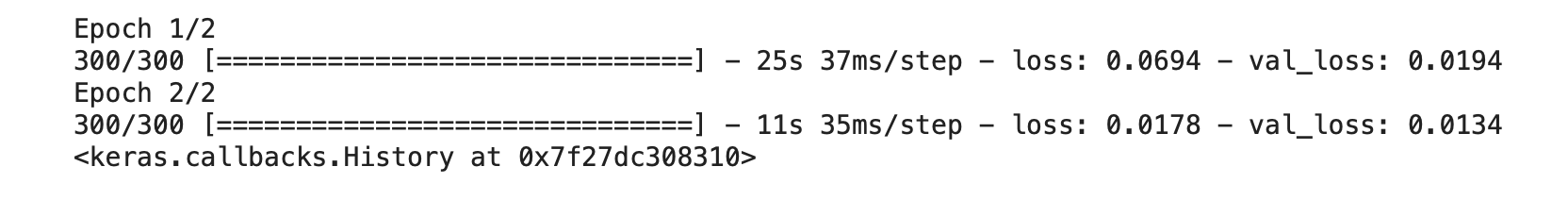
Here, we run our model only for two epochs but you can change this number according to your problem statement. Can you think 🤔 what happens when we change the number of epochs? Please think about it and I will explain this in the last of the article.

Evaluating the model

Finally, we will evaluate our trained model on the testing dataset, which we have created in the above section of loading our dataset. 

# Final evaluation of the model
pred = model.predict(x_test_noisy)

pred.shape

Output:

(10000, 784)

X_test.shape

Output:

(10000, 784)

X_test = numpy.reshape(X_test, (10000,28,28)) *255
pred = numpy.reshape(pred, (10000,28,28)) *255
x_test_noisy = numpy.reshape(x_test_noisy, (-1,28,28)) *255
plt.figure(figsize=(20, 4))
print("Test Images")
for i in range(10,20,1):
    plt.subplot(2, 10, i+1)
    plt.imshow(X_test[i,:,:], cmap='gray')
    curr_lbl = y_test[i]
    plt.title("(Label: " + str(curr_lbl) + ")")
plt.show()    
plt.figure(figsize=(20, 4))
print("Test Images with Noise")
for i in range(10,20,1):
    plt.subplot(2, 10, i+1)
    plt.imshow(x_test_noisy[i,:,:], cmap='gray')
plt.show()    
plt.figure(figsize=(20, 4))
print("Reconstruction of Noisy Test Images")
for i in range(10,20,1):
    plt.subplot(2, 10, i+1)
    plt.imshow(pred[i,:,:], cmap='gray')  
plt.show()

Output:

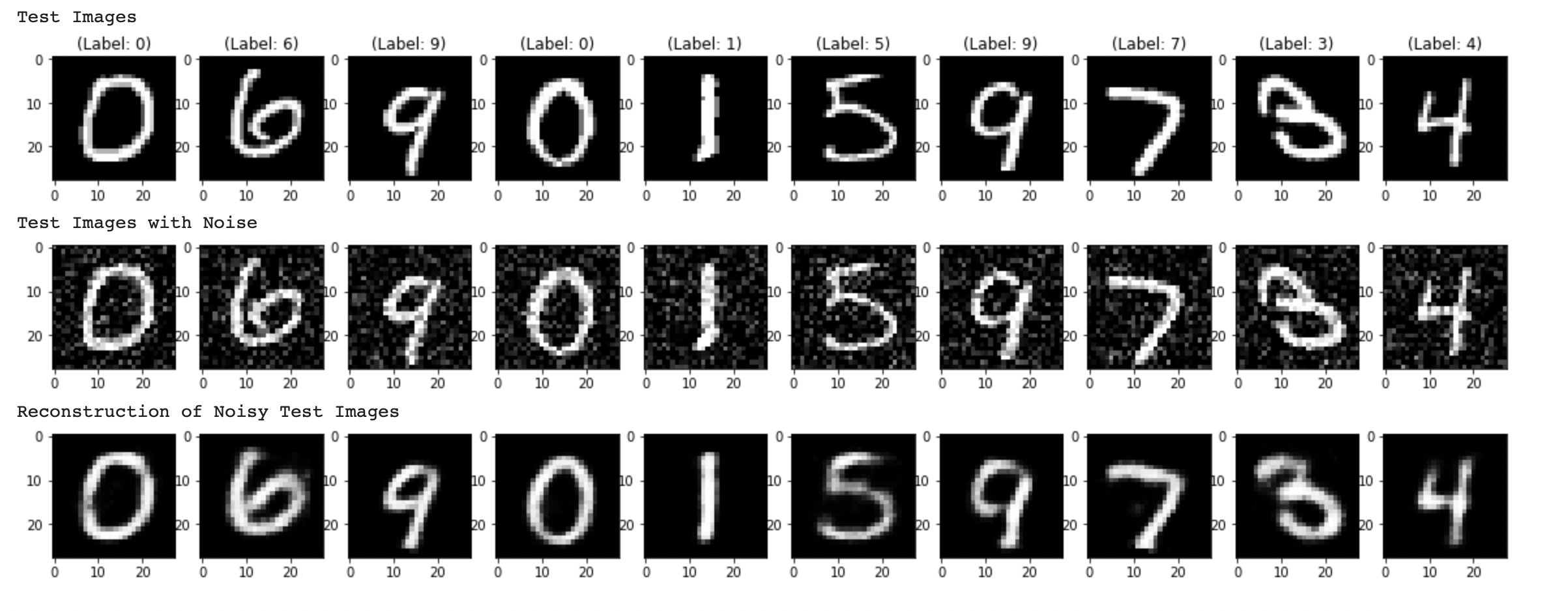
In the above output, the images in the:

• The first row is for original test images,
• The second row is for noisy images, and
• The third row is for cleaned (reconstructed) images.

See how the cleaned images are similar to the original images.

But if you closely look at the reconstructed image, then it might be seen as somewhat blurry. So can you think 🤔 some of the possible reasons why these images are blurred in the output of the decoder network. One of the possible reasons for this blurriness in the reconstructed images is to use fewer epochs while training our model. Therefore, now it’s your task to increase the value of the number of epochs and then again observed these images and also compare with these.

 If we want to summarize the whole process in one image, the image below is the best for that.

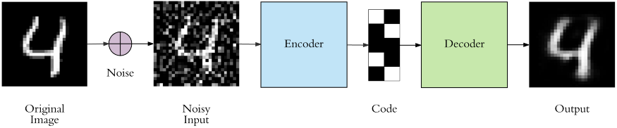
                                                            Image Source: Link

This ends our implementation!  🥳

Congratulations 👏

In this, tutorial, you have built an autoencoder model, which can successfully clean very noisy images, which it has never seen before (we used the test dataset). Obviously, there are some non-recovered distortions in these images. Yet, if you consider how deformed the noisy images are, we can say that our model is pretty successful in recovering the distorted images.

Off the top of my head, you can consider extending this autoencoder and embed it into a photo enhancement app, which can increase the clarity and crispiness of the photos.

This ends today’s discussion on the Beginner’s project of Deep Learning. If you have not understood either the concept or the code which I mentioned in this article, you can freely comment in the comment box below.

Other Blog Posts by Me

You can also check my previous blog posts.

Previous Data Science Blog posts.

LinkedIn

Here is my Linkedin profile in case you want to connect with me. I’ll be happy to be connected with you.

Email

For any queries, you can mail me on [email protected]

Conclusion

Thanks for reading!

I hope that you have enjoyed the article. If you like it, share it with your friends also. Something not mentioned or want to share your thoughts? Feel free to comment below And I’ll get back to you. 😉

Chirag Goyal

I am a B.Tech. student (Computer Science major) currently in the pre-final year of my undergrad. My interest lies in the field of Data Science and Machine Learning. I have been pursuing this interest and am eager to work more in these directions. I feel proud to share that I am one of the best students in my class who has a desire to learn many new things in my field.