A Beginners Guide to Machine Learning: Binary Classification of legendary Pokemon using multiple ML algorithms

This article was published as a part of the Data Science Blogathon

INTRODUCTION

Machine Learning is widely used across different problems in real-world scenarios. One of the major problems includes classification. Classification can be either binary or multi-class classification. In this article, we will dive deep into binary classification. We will first understand the binary classification and then apply different ML algorithms to see how accurately we can classify the target.

For this tutorial, I will be using the Pokemon stats dataset. Here we have stats of all the pokemon and we will try to accurately classify if the pokemon is legendary or not. In case you didn’t know, legendary pokemon are the ones who are very rare and powerful. We would love to see if these features, the stats are helping us to classify them.

Source: https://makeameme.org/meme/when-you-catch-59de4d

WHAT IS CLASSIFICATION?

In the Machine Learning world, classification refers to separating data to separate class labels. For a particular row in our dataset or values of features, we are interested in associating them to a particular target value. This is widely used in many applications like to say if you got spam mail or not. Is the image fake or not. If there are more than two class labels we call them multi-class classification.

In our case, we deal with only two classes Legendary or Not Legendary pokemon. So we have a binary classification problem. The question is how do we actually measure the accuracy. We have a confusion matrix here by Robert Alterman, which helps us tell if the classification we made is correct or wrong. This image here is one of the best ways to visualize legendary pokemon’s confusion matrix.

Source: https://towardsdatascience.com/gotta-classify-em-all-5f341d0c0c2

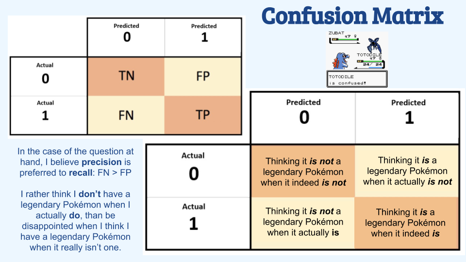
In the first diagonal of our confusion matrix, we can find the values that are perfectly predicted. Adding them and dividing with all values inside the matrix able gives us the accuracy of prediction.

Now let’s dive deep into different machine learning algorithms. In this tutorial, my intention is to show you the coding of each algorithm. The complete pre-processing and encoding with all codes are available in this COLAB link.

OUR DATASET:

The dataset is available here.

For the classification problem, we have used this dataset which has a Legendary column that tells us if the pokemon is legendary or not with True or False. We use Label encoding and encode them True as 1 and False as 0 before jumping into the next steps. Columns #, Name, Type 1, and Type 2 are not required and are removed from the dataset as part of preprocessing step. The final dataset used for ML algorithms looks like this:

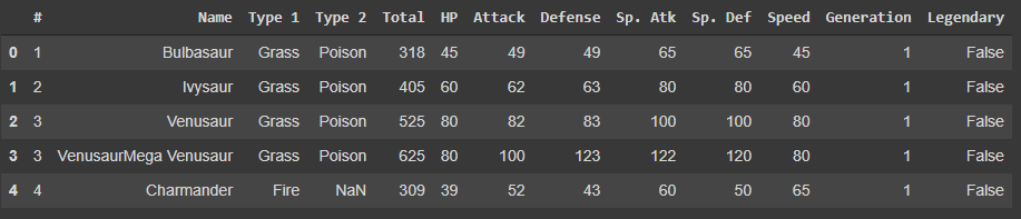
We can see here 8 columns are used as features and the last column is our Legendary which stands as the target variable to be predicted.

EXPLORATORY DATA ANALYSIS:

1. What is the distribution of different types of pokemon?

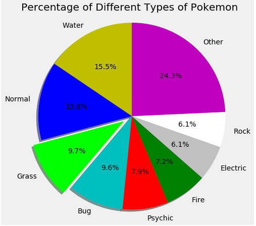
As we can see here Water pokemon are very common compared to all rest of them. Rock and electric pokemon are found less.

2. How correlated are each pokemon features?

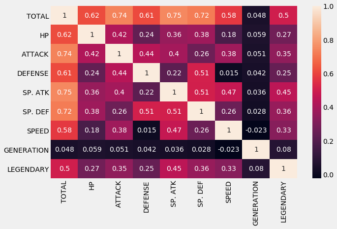
From the heatmap, it can be seen that there is not much correlation between the attributes of the pokemon. The highest we can see is the correlation between Special Attack and the Total.

3. Attack vs Defence for Fire Pokemons in each generation:

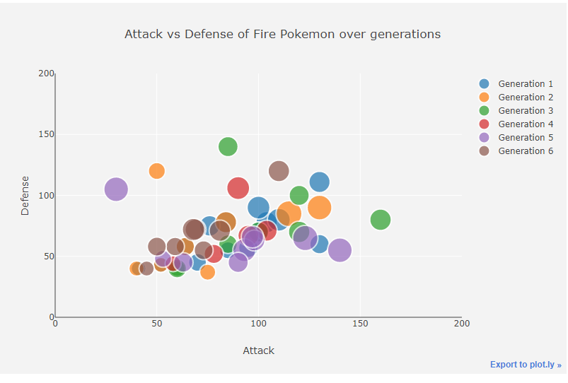
Generation 5 tends to have a lower defense. One of the 5th gen pokemon is the best attacker.

MACHINE LEARNING ALGORITHMS:

 

Source: https://miro.medium.com/max/1400/1*j7dwLFVWjLVRPQFTjMsmgg.jpeg

Logistic Regression:

Logistic regression is widely used for binary classification. It uses the logit function for the outcome. A probability is generated in output and it is classified into 0 or 1, by using the sigmoid activation function. The sigmoid function is given as:

Y = 1 / 1+e ^-z

from sklearn.metrics import accuracy_score
from sklearn.linear_model import LogisticRegression
lr = LogisticRegression()
lr.fit(X_train,Y_train)
Y_pred_lr = lr.predict(X_test)
score_lr = round(accuracy_score(Y_pred_lr,Y_test)*100,2)
print("The accuracy score we have achieved using Logistic Regression is: "+str(score_lr)+" %")

The accuracy score achieved using Logistic Regression is: 93.12 %

Gaussian Naive Bayes:

Naive Bayes is a probabilistic algorithm that makes use of the Bayes Theorem. We can give it as,

The probability of A, if B is true, is equal to the probability of B, if A is true, multiplied with the probability of A is true, divided by the probability of B is true.

from sklearn.naive_bayes import GaussianNB
nb = GaussianNB()
nb.fit(X_train,Y_train)
Y_pred_nb = nb.predict(X_test)
score_nb = round(accuracy_score(Y_pred_nb,Y_test)*100,2)
print("The accuracy score we have achieved using Naive Bayes is: "+str(score_nb)+" %")

The accuracy score achieved using Naive Bayes is: 91.88 %

Support Vector Machines:

SVM are supervised ML algorithms that are used to solve classification problems. We draw a hyperplane trying to separate two different classes here. More complex data, we can produce better results using the SVM algorithm. The algorithm can train large datasets but tends to be slower in nature.

from sklearn import svm
sv = svm.SVC(kernel='linear')
sv.fit(X_train, Y_train)
Y_pred_svm = sv.predict(X_test)
score_svm = round(accuracy_score(Y_pred_svm,Y_test)*100,2)
print("The accuracy score we have achieved using Linear SVM is: "+str(score_svm)+" %")

The accuracy score achieved using Linear SVM is: 94.38 %

K-Nearest Neighbours:

K-NN is a nearest neighbour classification algorithm. It tries to assign the points nearest to a neighbour. Voting happens in KNN and the neighbour near to points wins the point. K here denotes the number of neighbours that are available in our model.

from sklearn.neighbors import KNeighborsClassifier
knn = KNeighborsClassifier(n_neighbors=7)
knn.fit(X_train,Y_train)
Y_pred_knn=knn.predict(X_test)
score_knn = round(accuracy_score(Y_pred_knn,Y_test)*100,2)
print("The accuracy score we have achieved using KNN is: "+str(score_knn)+" %")

The accuracy score achieved using KNN is: 96.25 %

Decision Tree:

Decision trees are similar to a question answering system, where it decides to which child it has to place the points based on a specific condition. It, basically, acts as a flow chart, splitting the data points into two categories at a time, from “trunk,” to “branches,” then “leaves,” where the data within each category split based upon similarity.

from sklearn.tree import DecisionTreeClassifier
max_accuracy = 0
for x in range(200):
    dt = DecisionTreeClassifier(random_state=x)
    dt.fit(X_train,Y_train)
    Y_pred_dt = dt.predict(X_test)
    current_accuracy = round(accuracy_score(Y_pred_dt,Y_test)*100,2)
    if(current_accuracy>max_accuracy):
        max_accuracy = current_accuracy
        best_x = x
#print(max_accuracy)
#print(best_x)
dt = DecisionTreeClassifier(random_state=best_x)
dt.fit(X_train,Y_train)
Y_pred_dt = dt.predict(X_test)
score_dt = round(accuracy_score(Y_pred_dt,Y_test)*100,2)
print("The accuracy score we have achieved using Decision Tree is: "+str(score_dt)+" %")

The accuracy score achieved using the Decision Tree is: 96.25 %

Random Forest:

Random forest is expanding of decision tree and it mainly fixes the decision tree’s drawback of unnecessarily forcing data points into a somewhat incorrect category.

It works by initially constructing decision trees with train data available, then fits unseen data within one of the trees as a “random forest.” It averages our data to connect it to the nearest tree on the data scaled.

from sklearn.ensemble import RandomForestClassifier
max_accuracy = 0

for x in range(2000):
    rf = RandomForestClassifier(random_state=x)
    rf.fit(X_train,Y_train)
    Y_pred_rf = rf.predict(X_test)
    current_accuracy = round(accuracy_score(Y_pred_rf,Y_test)*100,2)
    if(current_accuracy>max_accuracy):
        max_accuracy = current_accuracy
        best_x = x
#print(max_accuracy)
#print(best_x)
rf = RandomForestClassifier(random_state=best_x)
rf.fit(X_train,Y_train)
Y_pred_rf = rf.predict(X_test)
score_rf = round(accuracy_score(Y_pred_rf,Y_test)*100,2)
print("The accuracy score we have achieved using Decision Tree is: "+str(score_rf)+" %")

The accuracy score achieved using the Decision Tree is: 98.12 %

XG-Boost:

XGBoost is mainly an implementation of gradient boosted decision trees used for speeding upscaling the performance in classification. 

import xgboost as xgb
xgb_model = xgb.XGBClassifier(objective="binary:logistic", random_state=42)
xgb_model.fit(X_train, Y_train)
Y_pred_xgb = xgb_model.predict(X_test)
score_xgb = round(accuracy_score(Y_pred_xgb,Y_test)*100,2)
print("The accuracy score we have achieved using XGBoost is: "+str(score_xgb)+" %")

The accuracy score achieved using XGBoost is: 96.88 %

Neural Network:

Neural networks are networks that mimic the human brain. Here we have constructed a neural network with 32 layered hidden layers. Since we have 8 features we take in as input dimensions. In the last layer, we use sigmoid as it is a binary classification problem. In between, we use ReLU as the activation function.

from keras.models import Sequential
from keras.layers import Dense
import tensorflow as tf
model = Sequential()
model.add(Dense(32,activation='relu',input_dim=8))
model.add(Dense(1,activation='sigmoid'))
model.compile(loss='binary_crossentropy',optimizer='adam',metrics=['accuracy'])
model.fit(X_train,Y_train,epochs=100, callbacks = tf.keras.callbacks.EarlyStopping(monitor='loss', patience=3))
Y_pred_nn = model.predict(X_test)
rounded = [round(x[0]) for x in Y_pred_nn]
Y_pred_nn = rounded
score_nn = round(accuracy_score(Y_pred_nn,Y_test)*100,2)
print("The accuracy score we have achieved using Neural Network is: "+str(score_nn)+" %")

The accuracy score achieved using Neural Network is: 90.62 %

RESULTS:

 

Source:https://heavy.com/games/2017/07/pokemon-go-fest-memes-tweets-reactions-disaster-pokemongo-chicago-jokes-funny-pics/

After running our pokemon features on various ML algorithms we could find that the XG-boost algorithm works well in our case with 96.88% accuracy followed by Random forest with 96.12%. Neural Networks aren’t that great for this current problem. But we may get better results by playing with different hidden layers or going for some complex models.

REFERENCES:

• https://www.kaggle.com/jashsheth5/binary-classification-with-sklearn-and-keras-95
• https://towardsdatascience.com/gotta-classify-em-all-5f341d0c0c2
• https://www.kaggle.com/thebrownviking20/intermediate-visualization-tutorial-using-plotly
• Image: https://unsplash.com/photos/DypO_XgAE4Y

CONCLUSION:

Source:https://www.usgamer.net/articles/pokemon-sword-and-shield-gives-you-an-up-close-look-at-a-pikachu-squirming-against-its-inevitable-end

About Me: I am a Research Student interested in the field of Deep Learning and Natural Language Processing and currently pursuing post-graduation in Artificial Intelligence.

Feel free to connect with me on:

1. Linkedin: https://www.linkedin.com/in/siddharth-m-426a9614a/

2. Github: https://github.com/Siddharth1698