This article was published as a part of the Data Science Blogathon
Introduction
OVERFITTING! We do not even spend a single day without encountering this situation and then try different options to get the correct accuracy of the model on the test dataset. But what if I tell you there exists a technique that inflicts a penalty on the model if it advances towards overfitting. Yeah, Yeah, you have heard it correct. We have some saviours that rescue our model from overfitting. Before moving further onto our rescuers, let us first understand overfitting with a real-world scenario:

Fig 1. Relocation from the hot region to the cold region
Suppose you have lived in a hot region all your life till graduation, and now for some reason, you have to move to a colder one. As soon as you move to a colder region, you feel under the weather because you need time to adapt to the new climate. The fact that you cannot simply adjust to the new environment can be called Overfitting.
In technical terms, overfitting is a condition that arises when we train our model too much on the training dataset that it focuses on noisy data and irrelevant features. Such a model runs with considerable accuracy on the training set but fails to generalize the attributes in the test set.
Why cannot we accept an Overfitted Model?
An overfitted model cannot recognize the unseen data and will fail terribly on given some new inputs. Understanding this with our previous example, if your body is fit to only one geographical area having a specific climate, then it cannot adapt to the new climate instantly.
For graphs, we can recognize overfitting by looking at the accuracy and loss during training and validation.
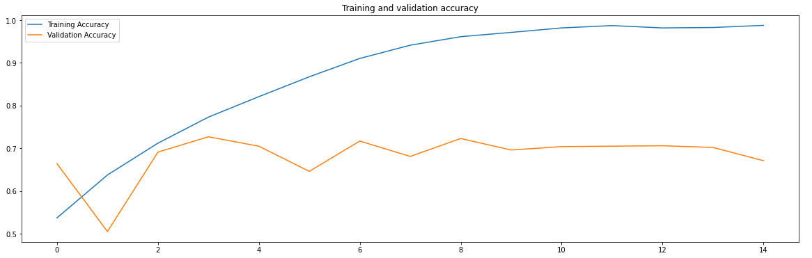
Fig 2. Training and Validation Accuracy
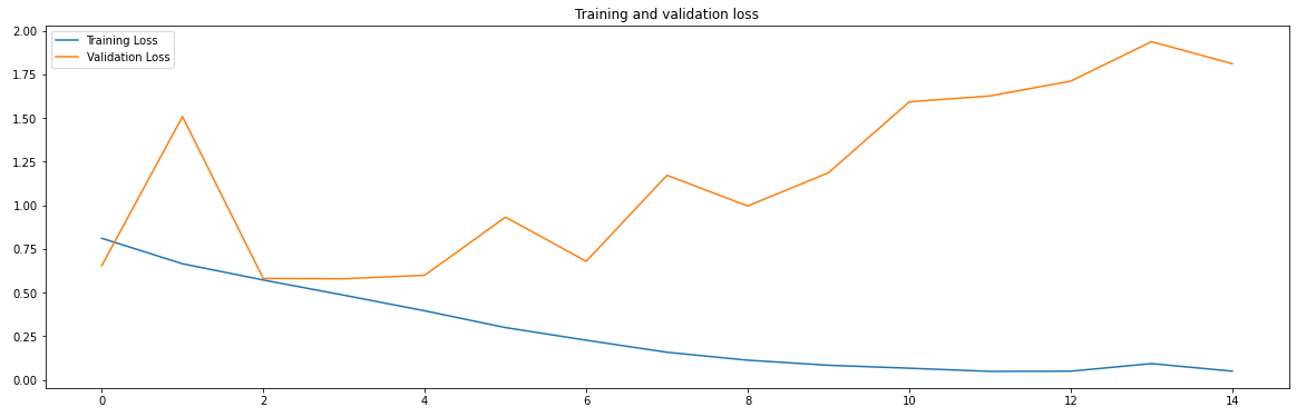
Fig 3. Training and Validation Loss
Mark that the training accuracy (in blue) strikes 100%, but the validation accuracy (in orange) reaches 70%. Training loss falls to 0 while the validation loss attains its minimum value just after the 2nd epoch. Training further enforces the model focus on noisy and irrelevant features for prediction, and thus the validation loss increases.
To get more insights about overfitting, it is fundamental to understand the role of variance and bias in overfitting:
What is Variance?
Variance tells us about the spread of the data points. It calculates how much a data point differs from its mean value and how far it is from the other points in the dataset.
What is Bias?
It is the difference between the average prediction and the target value.
The relationship of bias and variance with overfitting and underfitting is as shown below:
Fig 4. Bias and Variance w.r.t Overfitting and Underfitting
Low bias and low variance will give a balanced model, whereas high bias leads to underfitting, and high variance lead to overfitting.
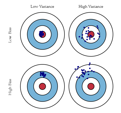
Fig 5. Bias Vs Variance
Low Bias: The average prediction is very close to the target value
High Bias: The predictions differ too much from the actual value
Low Variance: The data points are compact and do not vary much from their mean value
High Variance: Scattered data points with huge variations from the mean value and other data points.
To make a good fit, we need to have a correct balance of bias and variance.
What is Regularization?
- Regularization is one of the ways to improve our model to work on unseen data by ignoring the less important features.
- Regularization minimizes the validation loss and tries to improve the accuracy of the model.
- It avoids overfitting by adding a penalty to the model with high variance, thereby shrinking the beta coefficients to zero.
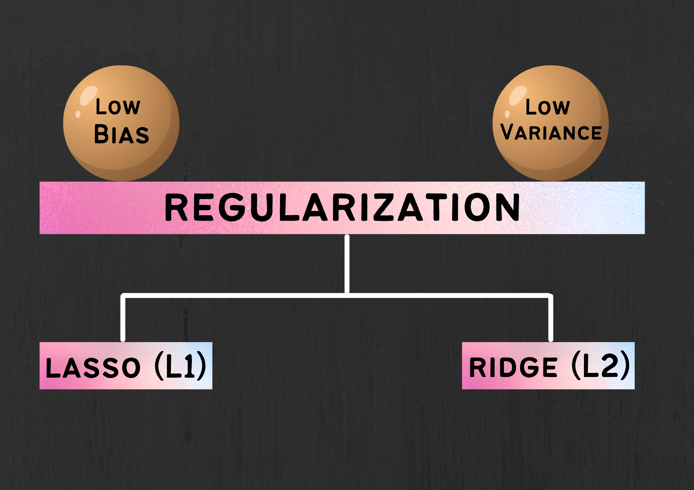
Fig 6. Regularization and its types
There are two types of regularization:
- Lasso Regularization
- Ridge Regularization
What is Lasso Regularization (L1)?
- It stands for Least Absolute Shrinkage and Selection Operator
- It adds L1 the penalty
- L1 is the sum of the absolute value of the beta coefficients
Cost function = Loss + λ + Σ ||w||
Here,
Loss = sum of squared residual
λ = penalty
w = slope of the curve
What is Ridge Regularization (L2)
- It adds L2 as the penalty
- L2 is the sum of the square of the magnitude of beta coefficients
Cost function = Loss + λ + Σ ||w||2
Here,
Loss = sum of squared residual
λ = penalty
w = slope of the curve
λ is the penalty term for the model. As λ increases cost function increases, the coefficient of the equation decreases and leads to shrinkage.
Now its time to dive into some code:
For comparing Linear, Ridge, and Lasso Regression I will be using a real estate dataset where we have to predict the house price of unit area.
Dataset looks like this:
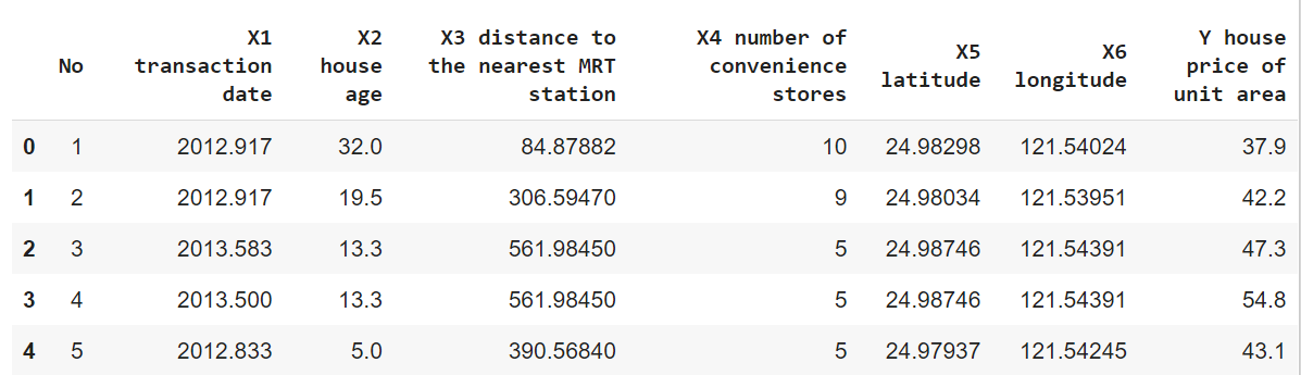
Fig 7. Real Estate Dataset
Dividing the dataset into train and test sets:
X = df.drop(columns = ['Y house price of unit area', 'X1 transaction date', 'X2 house age'])
Y = df['Y house price of unit area']
x_train, x_test,y_train, y_test = train_test_split(X, Y, test_size = 0.2, random_state = 42)
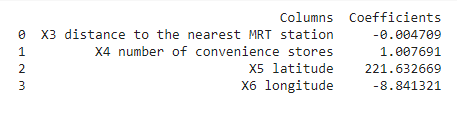
Fitting the model on Linear Regression:
lin_reg = LinearRegression()
lin_reg.fit(x_train, y_train)
lin_reg_y_pred = lin_reg.predict(x_test)
mse = mean_squared_error(y_test, lin_reg_y_pred)
print(mse)
The Mean Square Error for Linear Regression is: 63.90493104709001
The coefficients of the columns for the Linear Regression model are:
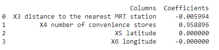
Fitting the model on Lasso Regression:
from sklearn.linear_model import Lasso
lasso = Lasso()
lasso.fit(x_train, y_train)
y_pred_lasso = lasso.predict(x_test)
mse = mean_squared_error(y_test, y_pred_lasso)
print(mse)
The Mean Square Error for Lasso Regression is: 67.04829587817319
The coefficients of the columns for the Linear Regression model are:
Fitting the model on Ridge Regression:
from sklearn.linear_model import Ridge
ridge = Ridge()
ridge.fit(x_train, y_train)
y_pred_ridge = ridge.predict(x_test)
mse = mean_squared_error(y_test, y_pred_ridge)
print(mse)
The Mean Square Error for Ridge Regression is: 66.07258621837418
The coefficients of the columns for the Linear Regression model are:
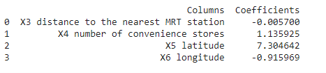
Comparing the coefficients of the Lasso and Ridge Regularization models
plt.figure(figsize=(30,6))
x = ['Linear', 'Lasso', 'Ridge']
y1 = np.array([-0.004709, -0.005994, 0.005700])
y2 = np.array([1.007691, 0.958896,  1.135925])
y3 = np.array([221.632669, 0.000000, 7.304642])
y4 = np.array([-8.841321, -0.000000, -0.915969])
fig, axes = plt.subplots(ncols=1, nrows=1)
plt.bar(x, y1, color = 'black')
plt.bar(x, y2, bottom=y1, color='b')
plt.bar(x, y3, bottom=y1+y2, color='g')
plt.bar(x, y4, bottom=y1+y2+y3, color='r')
plt.xlabel("Models")
plt.ylabel("Coefficients")
plt.legend(["X3", "X4", "X5", "X6"])
plt.title("Comparing coefficients of different models")
axes.set_xticklabels(['Linear', 'Lasso', 'Ridge'])
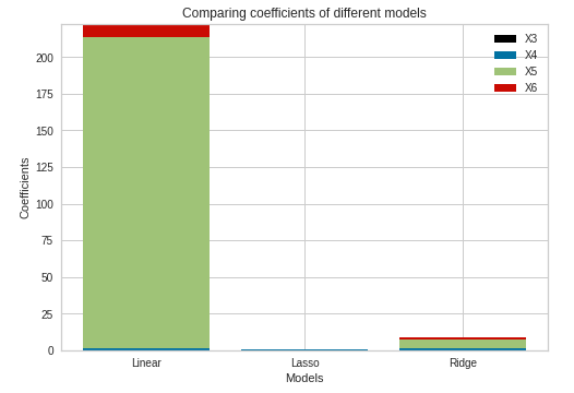
Fig 11. Comparison of Beta Coefficients
Inspecting the coefficients, we can see that Lasso and Ridge Regression had shrunk the coefficients, and thus the coefficients are close to zero. On the contrary, Linear Regression still has a substantial value of the coefficient for the X5 column.\
Comparing Lasso and Ridge Regularization techniques

Conclusion
We learned two different types of regression techniques, namely Lasso and Ridge Regression which can be proved effective for overfitting. These techniques make a good fit model by adding a penalty and shrinking the beta coefficients. It is necessary to have a correct balance of the Bias and Variance to control overfitting.
Yayyy! You’ve made it to the end of the article and successfully gotten the hang of these topics of Bias and Variance, Overfitting and Underfitting, and Regularization techniques.😄
Happy Learning! 😊
I’d be obliged to receive any comments, suggestions, or feedback.
You can find the complete code here.
Stay tuned for upcoming blogs!
Connect on LinkedIn: https://www.linkedin.com/in/rashmi-manwani-a13157184/
Connect on Github: https://github.com/Rashmiii-00
Fig 5: http://scott.fortmann-roe.com/docs/BiasVariance.html
About the Author:
Rashmi Manwani
Passionate to learn about Machine Learning topics and their implementation. Thus, finding my way to develop a strong knowledge of the domain by writing appropriate articles on Data Science topics.
The media shown in this article on Interactive Dashboard using Bokeh are not owned by Analytics Vidhya and are used at the Author’s discretion.


