Generative Adversarial Networks(GANs): End-to-End Introduction
Introduction
There are many ways a machine can be taught to generate an output on unseen data. The technological advancement in different sectors has left everyone shocked. we are now at a point where deep learning and neural networks are so powerful that can generate a new human face from scratch that does not exist before but looks real based on some trained data. The technique is none other than GAN(Generative Adversarial Network) which is our topic of study. Let’s look at the table of content to understand the main topics we will cover.
This article was published as a part of the Data Science Blogathon
Table of contents
- What are Generative Adversarial Networks (GANs)?
- Applications of Generative Adversarial Networks (GANs)
- Components of Generative Adversarial Networks (GANs)
- Training & Prediction of Generative Adversarial Networks (GANs)
- Generative Adversarial Networks (GANs) Loss Function
- Challenges Faced by Generative Adversarial Networks (GANs)
- Different Types of Generative Adversarial Networks (GANs)
- Steps to Implement Basic GAN
- Practical Implementation of Generative Adversarial Networks (GANs) on MNIST Dataset
What are Generative Adversarial Networks (GANs)?
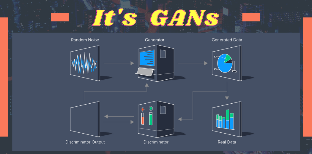
Generative Adversarial Networks (GANs) were developed in 2014 by Ian Goodfellow and his teammates. GAN is basically an approach to generative modeling that generates a new set of data based on training data that look like training data. GANs have two main blocks(two neural networks) which compete with each other and are able to capture, copy, and analyze the variations in a dataset. The two models are usually called Generator and Discriminator which we will cover in Components on GANs.
GAN let’s break it into separate three parts
- Generative – To learn a generative model, which describes how data is generated in terms of a probabilistic model. In simple words, it explains how data is generated visually.
- Adversarial – The training of the model is done in an adversarial setting.
- Networks – use deep neural networks for training purposes.
The generator network takes random input (typically noise) and generates samples, such as images, text, or audio, that resemble the training data it was trained on. The goal of the generator is to produce samples that are indistinguishable from real data.
The discriminator network, on the other hand, tries to distinguish between real and generated samples. It is trained with real samples from the training data and generated samples from the generator. The discriminator’s objective is to correctly classify real data as real and generated data as fake.
The training process involves an adversarial game between the generator and the discriminator. The generator aims to produce samples that fool the discriminator, while the discriminator tries to improve its ability to distinguish between real and generated data. This adversarial training pushes both networks to improve over time.
As training progresses, the generator becomes more adept at producing realistic samples, while the discriminator becomes more skilled at differentiating between real and generated data. Ideally, this process converges to a point where the generator is capable of generating high-quality samples that are difficult for the discriminator to distinguish from real data.
GANs have demonstrated impressive results in various domains, such as image synthesis, text generation, and even video generation. They have been used for tasks like generating realistic images, creating deepfakes, enhancing low-resolution images, and more. GANs have greatly advanced the field of generative modeling and have opened up new possibilities for creative applications in artificial intelligence.
Why GANs was Developed?
Machine learning algorithms and neural networks can easily be fooled to misclassify things by adding some amount of noise to data. After adding some amount of noise, the chances of misclassifying the images increase. Hence the small rise that, is it possible to implement something that neural networks can start visualizing new patterns like sample train data. Thus GANs were built that generate new fake results similar to the original.
Applications of Generative Adversarial Networks (GANs)
- Generate new data from available data – It means generating new samples from an available sample that is not similar to a real one.
- Generate realistic pictures of people that have never existed.
- Gans is not limited to Images, It can generate text, articles, songs, poems, etc.
- Generate Music by using some clone Voice – If you provide some voice then GANs can generate a similar clone feature of it. In this research paper, researchers from NIT in Tokyo proposed a system that is able to generate melodies from lyrics with help of learned relationships between notes and subjects.
- Text to Image Generation (Object GAN and Object Driven GAN)
- Creation of anime characters in Game Development and animation production.
- Image to Image Translation – We can translate one Image to another without changing the background of the source image. For example, Gans can replace a dog with a cat.
- Low resolution to High resolution – If you pass a low-resolution Image or video, GAN can produce a high-resolution Image version of the same.
- Prediction of Next Frame in the video – By training a neural network on small frames of video, GANs are capable to generate or predict a small next frame of video. For example, you can have a look at below GIF
- Interactive Image Generation – It means that GANs are capable to generate images and video footage in an art form if they are trained on the right real dataset.
- Speech – Researchers from the College of London recently published a system called GAN-TTS that learns to generate raw audio through training on 567 corpora of speech data.
Components of Generative Adversarial Networks (GANs)
What is Geometric Intuition behind the working of GANs?
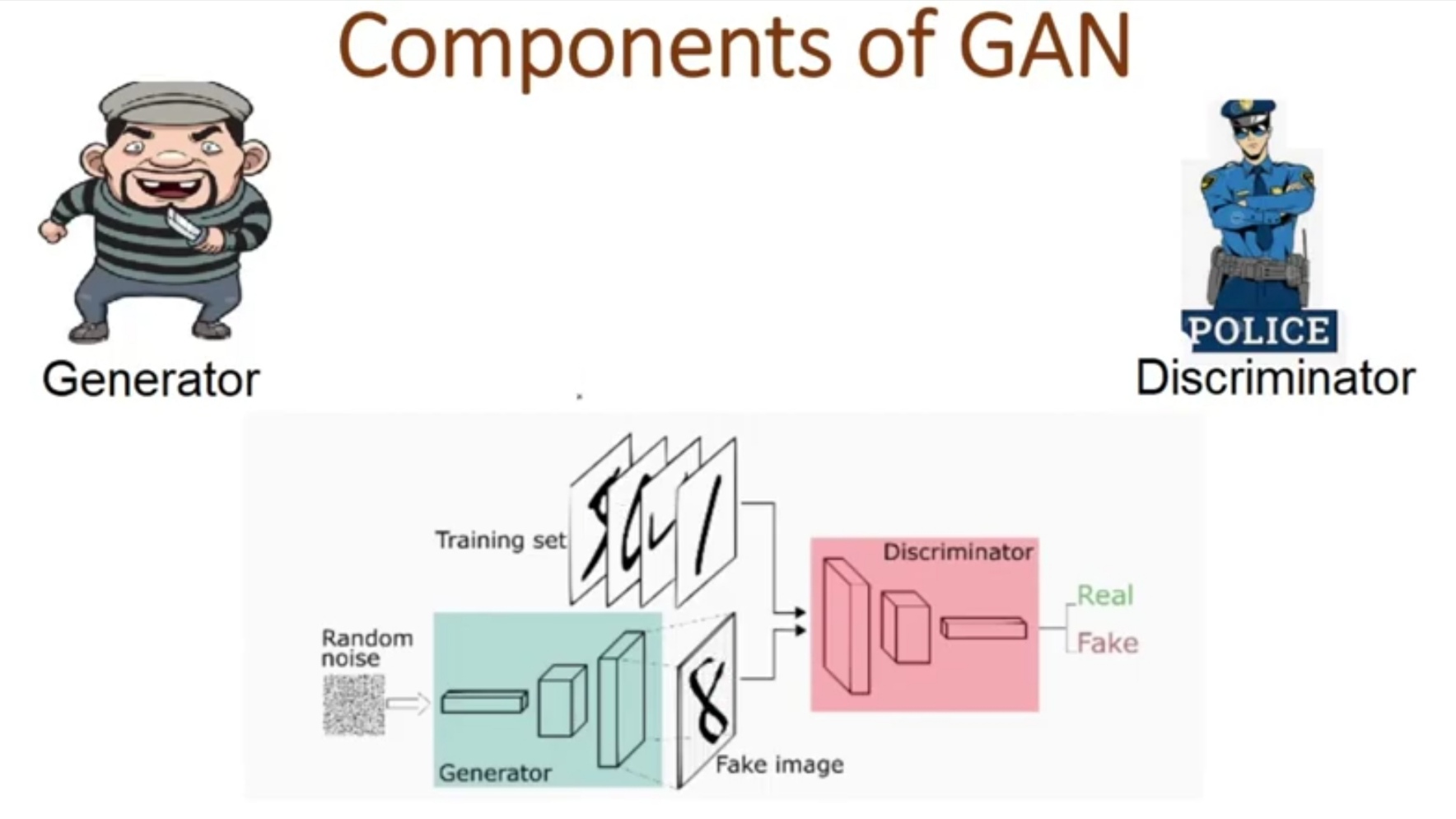
Two major components of GANs are Generator and Discriminator. The role of the generator is like a thief to generate the fake samples based on the original sample and make the discriminator fool to understand Fake as real. On the other hand, a Discriminator is like a Police whose role is to identify the abnormalities in the samples created by Generator and classify them as Fake or real. This competition between both the component goes on until the level of perfection is achieved where Generator wins making a Discriminator fool on fake data.
Now let us understand, what is this two-component to understand the training process of GAN intuitively.
Discriminator
It is a supervised approach means It is a simple classifier that predicts data is fake or real. It is trained on real data and provides feedback to a generator.
Generator
It is an unsupervised learning approach. It will generate data that is fake data based on original(real) data. It is also a neural network that has hidden layers, activation, loss function. Its aim is to generate the fake image based on feedback and make the discriminator fool that it cannot predict a fake image. And when the discriminator is made a fool by the generator, the training stops and we can say that a generalized GAN model is created.
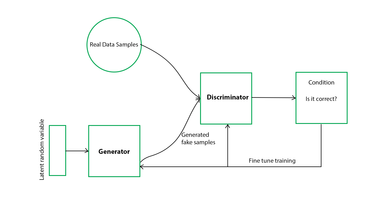
Image 2
Here the generative model captures the distribution of data and is trained in such a manner to generate the new sample that tries to maximize the probability of the discriminator to make a mistake(maximize discriminator loss). The discriminator on other hand is based on a model that estimates the probability that the sample it receives is from training data not from the generator and tries to classify it accurately and minimize the GAN accuracy. Hence the GAN network is formulated as a minimax game where the Discriminator is trying to minimize its reward V(D, G) and the generator is trying to maximize the Discriminator loss.
Now you might be wondering how is an actual architecture of GAN, and how two neural networks are build and training and prediction is done? To simplify it have a look at the below general architecture of GAN.
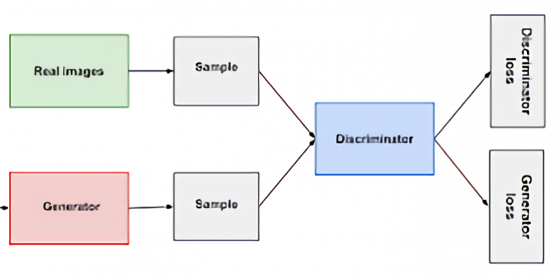
Image 3
We know that both components are neural networks. we can see that generator output is directly connected to the input of the discriminator. And discriminator predicts it and through backpropagation, the generator receives a feedback signal to update weights and improve performance. The discriminator is a feed-forward neural network.
Training & Prediction of Generative Adversarial Networks (GANs)
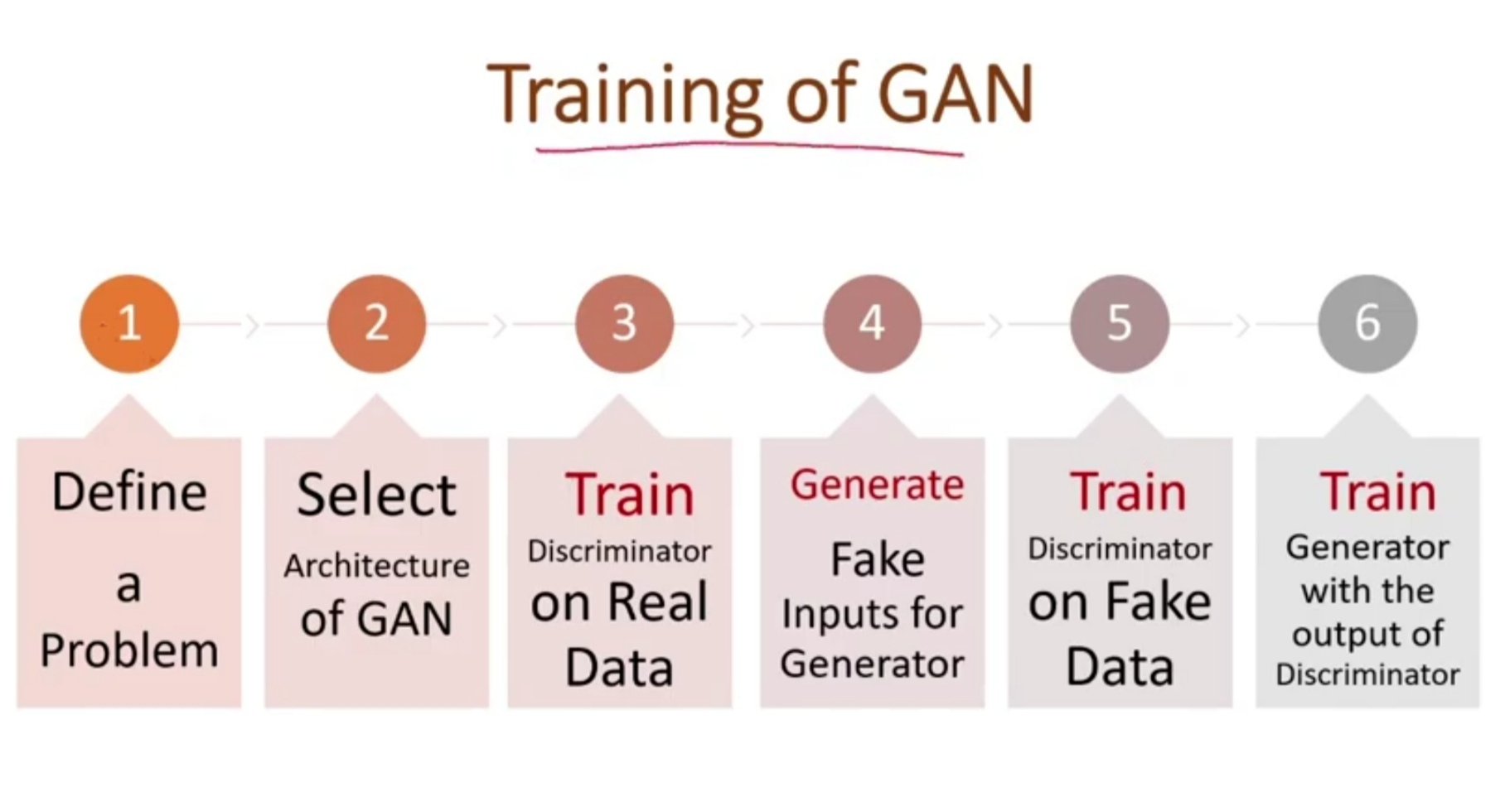
We know the geometric intuition of GAN, Now let us understand the training of Gan. In this section training of Generator and Discriminator will separately be clear to you.
Step-1) Define a Problem
The problem statement is key to the success of the project so the first step is to define your problem. GANs work with a different set of problems you are aiming so you need to define What you are creating like audio, poem, text, Image is a type of problem.
Step-2) Select Architecture of GAN
There are many different types of GAN, that we will study further. we have to define which type of GAN architecture we are using.
Step-3) Train Discriminator on Real Dataset
Now Discriminator is trained on a real dataset. It is only having a forward path, no backpropagation is there in the training of the Discriminator in n epochs. And the Data you are providing is without Noise and only contains real images, and for fake images, Discriminator uses instances created by the generator as negative output. Now, what happens at the time of discriminator training.
- It classifies both real and fake data.
- The discriminator loss helps improve its performance and penalize it when it misclassifies real as fake or vice-versa.
- weights of the discriminator are updated through discriminator loss.
Step-4) Train Generator
Provide some Fake inputs for the generator(Noise) and It will use some random noise and generate some fake outputs. when Generator is trained, Discriminator is Idle and when Discriminator is trained, Generator is Idle. During generator training through any random noise as input, it tries to transform it into meaningful data. to get meaningful output from the generator takes time and runs under many epochs. steps to train a generator are listed below.
- get random noise and produce a generator output on noise sample
- predict generator output from discriminator as original or fake.
- we calculate discriminator loss.
- perform backpropagation through discriminator, and generator both to calculate gradients.
- Use gradients to update generator weights.
Step-5) Train Discriminator on Fake Data
The samples which are generated by Generator will pass to Discriminator and It will predict the data passed to it is Fake or real and provide feedback to Generator again.
Step-6) Train Generator with the output of Discriminator
Again Generator will be trained on the feedback given by Discriminator and try to improve performance.
This is an iterative process and continues running until the Generator is not successful in making the discriminator fool.
Generative Adversarial Networks (GANs) Loss Function
I hope that the working of the GAN network is completely understandable and now let us understand the loss function it uses and minimize and maximize in this iterative process. The generator tries to minimize the following loss function while the discriminator tries to maximize it. It is the same as a minimax game if you have ever played.
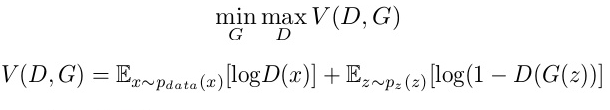
- D(x) is the discriminator’s estimate of the probability that real data instance x is real.
- Ex is the expected value over all real data instances.
- G(z) is the generator’s output when given noise z.
- D(G(z)) is the discriminator’s estimate of the probability that a fake instance is real.
- Ez is the expected value over all random inputs to the generator (in effect, the expected value over all generated fake instances G(z)).
- The formula is derived from cross-entropy between
Challenges Faced by Generative Adversarial Networks (GANs)
- The problem of stability between generator and discriminator. We do not want that discriminator should be too strict, we want to be lenient
- Problem to determine the positioning of objects. suppose in a picture we have 3 horse and generator have created 6 eyes and 1 horse.
- The problem in understanding the global objects – GANs do not understand the global structure or holistic structure which is similar to the problem of perspective. It means sometimes GAN generates an image that is unrealistic and cannot be possible.
- A problem in understanding the perspective – It cannot understand the 3-d images and if we train it on such types of images then it will fail to create 3-d images because today GANs are capable to work on 1-d images.
Different Types of Generative Adversarial Networks (GANs)
1) DC GAN – It is a Deep convolutional GAN. It is one of the most used, powerful, and successful types of GAN architecture. It is implemented with help of ConvNets in place of a Multi-layered perceptron. The ConvNets use a convolutional stride and are built without max pooling and layers in this network are not completely connected.
2) Conditional GAN and Unconditional GAN (CGAN) – Conditional GAN is deep learning neural network in which some additional parameters are used. Labels are also put in inputs of Discriminator in order to help the discriminator to classify the input correctly and not easily full by the generator.
3) Least Square GAN(LSGAN) – It is a type of GAN that adopts the least-square loss function for the discriminator. Minimizing the objective function of LSGAN results in minimizing the Pearson divergence.
4) Auxilary Classifier GAN(ACGAN) – It is the same as CGAN and an advanced version of it. It says that the Discriminator should not only classify the image as real or fake but should also provide the source or class label of the input image.
5) Dual Video Discriminator GAN – DVD-GAN is a generative adversarial network for video generation built upon the BigGAN architecture. DVD-GAN uses two discriminators: a Spatial Discriminator and a Temporal Discriminator.
6) SRGAN – Its main function is to transform low resolution to high resolution known as Domain Transformation.
7) Cycle GAN
It is released in 2017 which performs the task of Image Translation. Suppose we have trained it on a horse image dataset and we can translate it into zebra images.
8) Info GAN – Advance version of GAN which is capable to learn to disentangle representation in an unsupervised learning approach.
Steps to Implement Basic GAN
- Importing all libraries
- Getting the Dataset
- Data Preparation – It includes various steps to accomplish like preprocessing data, scaling, flattening, and reshaping the data.
- Define the function Generator and Discriminator.
- Create a Random Noise and then create an Image with Random Noise.
- Setting Parameters like defining epoch, batch size, and Sample size.
- Define the function of generating Sample Images.
- Train Discriminator then trains Generator and it will create Images.
- Will see what clarity of Images is created by Generator.
Practical Implementation of Generative Adversarial Networks (GANs) on MNIST Dataset
Now we will follow all the above steps and make our hands dirty by implementing GAN on a very popular dataset known as MNIST Dataset.
About Dataset
MNIST Dataset is a very popular dataset of hand-written digits images between 0 to 9 in grayscale form of size 28*28. And a total of 60000 images of such small square images is present in the MNIST dataset.
Our aim is to train the Discriminator Model with MNIST dataset and with some Noise and after providing some sample noise same as MNIST to Generator model to generate the same information as MNIST dataset that gives feels exactly or original images but are actually generated by Generator model. let’s get started with importing the libraries we need.
Importing libraries
Import libraries are helpful for preprocessing, transforming, and creating a neural network model.
import numpy as np
import pandas as pd
import matplotlib.pyplot as plt
import os
import tensorflow as tf
from tensorflow.keras.layers import Input, Dense, LeakyReLU, Dropout, BatchNormalization
from tensorflow.keras.models import Model
from tensorflow.keras.optimizers import SGD, Adam
Loading MNIST Dataset
When we load the in-built dataset from any library then most of the time It is already splitted into train and test set so we will load a dataset into two different forms.
mnist = tf.keras.datasets.mnist
(x_train, y_train), (x_test, y_test) = mnist.load_data()
# Scale the inputs in range of (-1, +1) for better training
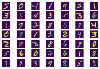
x_train, x_test = x_train / 255.0 * 2 - 1, x_test / 255.0 * 2 - 1If you want to plot some example images from the dataset then you can simply plot it from the training dataset using matplotlib.
for i in range(49):
  plt.subplot(7, 7, i+1)
  plt.axis("off")
  #plot raw pixel data
  plt.imshow(x_train[i])
plt.show()
If you print the shape of the dataset then train data has 60000 images of 28*28 size and test data has 10000 images of 28*28 size.
Flattening and Scaling the data
As the dimension of the dataset is 3 so we will flatten it to 2 dimensions and 28*28 means 684 and get converted to 60000 by 684.
N, H, W = x_train.shape  #number, height, width
D = H * W   #dimension (28, 28)
x_train = x_train.reshape(-1, D)
x_test = x_test.reshape(-1, D)
Defining Generator Model
Here we define a function to develop a deep convolutional Neural network. latent dimension is a variable that defines the number of inputs to the model. We define the input layer, three hidden layers followed by Batch normalization, and activation function as Leaky RELU and an output layer with activation function as tanh because a range of Image pixel is between -1 and +1.
# Defining Generator Model
latent_dim = 100
def build_generator(latent_dim):
  i = Input(shape=(latent_dim,))
  x = Dense(256, activation=LeakyReLU(alpha=0.2))(i)
  x = BatchNormalization(momentum=0.7)(x)
  x = Dense(512, activation=LeakyReLU(alpha=0.2))(x)
  x = BatchNormalization(momentum=0.7)(x)
  x = Dense(1024, activation=LeakyReLU(alpha=0.2))(x)
  x = BatchNormalization(momentum=0.7)(x)
  x = Dense(D, activation='tanh')(x)  #because Image pixel is between -1 to 1.
  model = Model(i, x)  #i is input x is output layer
  return model
Why do we use Leaky RELU?
Leaky relu helps the Gradient flow easily through the neural network architecture.
- The ReLU activation function only takes the maximum value between input and zero. If we use ReLU then it is a chance that the network can get stuck in a state known as Dying State. If this happens then it produces nothing other than zero for all outputs.
- Our aim is to get the value of gradient from Discriminator to make the generator work, and If the network gets stuck then learning will not happen.
- Leaky ReLU uses a parameter known as alpha to control negative values and never zero passes. If the input is positive then it will exhibit a positive value, and if receive negative then multiply it with alpha and allow some negative value to pass through the network.

Why Batch Normalization?
It has the effect of stabilizing the training process by standardizing activations from the prior layer to have zero mean and unit variance. Batch Normalization has become a staple while training deep convolutional Networks and GANs are no different from it.
Applying batch norm directly to all layers resulted in sample oscillation and model instability.
Defining Discriminator Model
Here we develop a simple Feed Forward Neural network for Discriminator where we will pass an image size. The activation function used is Leaky ReLU and you know the reason for it and sigmoid is used in the output layer for binary classification problems to classify Images as real or Fake.
def build_discriminator(img_size):
  i = Input(shape=(img_size,))
  x = Dense(512, activation=LeakyReLU(alpha=0.2))(i)
  x = Dense(256, activation=LeakyReLU(alpha=0.2))(x)
  x = Dense(1, activation='sigmoid')(x)
  model = Model(i, x)
  return model
Compile Models
Now it’s time to compile both the defined components of GANs
# Build and compile the discriminator
discriminator = build_discriminator(D)
discriminator.compile ( loss='binary_crossentropy', optimizer=Adam(0.0002, 0.5), metrics=['accuracy'])
# Build and compile the combined model
generator = build_generator(latent_dim)
Represent Noise Sample
Now we will create input to represent noise samples from latent space. And we pass this noise to a generator to generate an Image. After this, we pass the generator Image to Discriminator and predict that it is Fake or real. In the initial phase, we do not want the discriminator to be trained and the image is Fake.
## Create an input to represent noise sample from latent space
z = Input(shape=(latent_dim,))
## Pass noise through a generator to get an Image
img = generator(z)
discriminator.trainable = False
fake_pred = discriminator(img)
Create Generator Model
It’s time to create a combined Generator model with noise input and feedback of discriminator that helps the generator to improve its performance.
combined_model_gen = Model(z, fake_pred)  #first is noise and 2nd is fake prediction
# Compile the combined model
combined_model_gen.compile(loss='binary_crossentropy', optimizer=Adam(0.0002, 0.5))
Defining Parameters for the training of GAN
Define epochs, batch size, and a sample period which means after how many steps the generator will create a sample. After this, we define the Batch labels as one and zero. One represents that image is real and zero represents the image is fake. And we also create two empty lists to store the loss of generator and discriminator. And very importantly we create an empty file in the working directory where the generated image through the generator will be saved.
batch_size = 32
epochs = 12000
sample_period = 200
ones = np.ones(batch_size)
zeros = np.zeros(batch_size)
#store generator and discriminator loss in each step or each epoch
d_losses = []
g_losses = []
#create a file in which generator will create and save images
if not os.path.exists('gan_images'):
  os.makedirs('gan_images')
Function to create Sample Images
Create a function that generates a grid of random samples from a generator and saves them to a file. In simple words, it will create random images on some epochs. We define the row size as 5 and column as also 5 so in a single iteration or on a single page it will generate 25 images.
def sample_images(epoch):
  rows, cols = 5, 5
  noise = np.random.randn(rows * cols, latent_dim)
  imgs = generator.predict(noise)
  # Rescale images 0 - 1
  imgs = 0.5 * imgs + 0.5
  fig, axs = plt.subplots(rows, cols)  #fig to plot img and axis to store
  idx = 0
  for i in range(rows):  #5*5 loop means on page 25 imgs will be there
    for j in range(cols):
      axs[i,j].imshow(imgs[idx].reshape(H, W), cmap='gray')
      axs[i,j].axis('off')
      idx += 1
  fig.savefig("gan_images/%d.png" % epoch)
  plt.close()
Train Discriminator and then Generator to generate Images
Now let’s start the training Discriminator. We have to pass real images means MNIST dataset as well some Fake Images to Discriminator to train it well that it is capable to classify images. After this, we create a random noise grid the same as of real image and pass it to a generator to generate a new image. After this, we calculate the loss of both models and in a generated image, we pass the label as one to fool the Discriminator to believe and check that it is capable to identify it as Fake or not.
#FIRST we will train Discriminator(with real imgs and fake imgs)
# Main training loop
for epoch in range(epochs):
  ###########################
  ### Train discriminator ###
  ###########################
  # Select a random batch of images
  idx = np.random.randint(0, x_train.shape[0], batch_size)
  real_imgs = x_train[idx]  #MNIST dataset
  # Generate fake images
  noise = np.random.randn(batch_size, latent_dim)  #generator to generate fake imgs
  fake_imgs = generator.predict(noise)
  # Train the discriminator
  # both loss and accuracy are returned
  d_loss_real, d_acc_real = discriminator.train_on_batch(real_imgs, ones)  #belong to positive class(real imgs)
  d_loss_fake, d_acc_fake = discriminator.train_on_batch(fake_imgs, zeros)  #fake imgs
  d_loss = 0.5 * (d_loss_real + d_loss_fake)
  d_acc  = 0.5 * (d_acc_real + d_acc_fake)
  #######################
  ### Train generator ###
  #######################
  noise = np.random.randn(batch_size, latent_dim)
  g_loss = combined_model_gen.train_on_batch(noise, ones)
  #Now we are trying to fool the discriminator that generate imgs are real that's why we are providing label as 1
  # do it again!
  noise = np.random.randn(batch_size, latent_dim)
  g_loss = combined_model_gen.train_on_batch(noise, ones)
  # Save the losses
  d_losses.append(d_loss)  #save the loss at each epoch
  g_losses.append(g_loss)
  if epoch % 100 == 0:
    print(f"epoch: {epoch+1}/{epochs}, d_loss: {d_loss:.2f},
      d_acc: {d_acc:.2f}, g_loss: {g_loss:.2f}")
  if epoch % sample_period == 0:
    sample_images(epoch)
We trained it on 12000 epochs, you can train on more epochs. It will take some time so better to use Kaggle or Google Colab GPU. And generated images will be saved with the name gan image followed by an epoch number in the defined directory.
Plot Loss Function
We have finished the training of GAN and let’s see what accuracy the Generator is capable of to make Discriminator Fool.
plt.plot(g_losses, label='g_losses')
plt.plot(d_losses, label='d_losses')
plt.legend()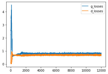
Check the results
Let’s plot the generated images at different epochs to see that after how many epochs the generator was capable to extract some information.
Plot the generated Image at zero epoch
from skimage.io import imread
a = imread('gan_images/0.png')
plt.imshow(a)
let’s see at the initial epoch what results in it being generated.
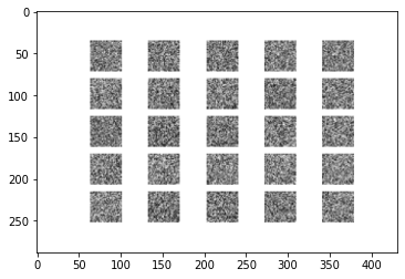
No information is extracted from the generator and the discriminator is intelligent enough to identify it as fake.
Plot Image Generated after training on 1000 epoch
from skimage.io import imread
a = imread('gan_images/10000.png')
plt.imshow(a)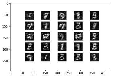
Now Generator is slowly being capable to extract some information that can be observed.
Plot Image Generated after training on 10000 Epochs
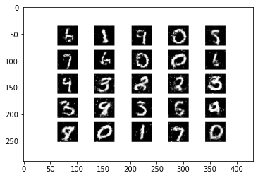
Now Generator is capable to build as it is an image as of MNIST dataset and there are high chances of the Discriminator being Fool.
Conclusion
Generative Adversarial Networks (GANs) represent a powerful paradigm in the field of machine learning, offering diverse applications and functionalities. This analysis of the table of contents highlights the comprehensive nature of GANs, covering their definition, applications, components, training methodologies, loss functions, challenges, variations, implementation steps, and practical demonstrations. GANs have demonstrated remarkable capabilities in generating realistic data, enhancing image processing, and facilitating creative applications. Despite their effectiveness, challenges such as mode collapse and training instability persist, necessitating ongoing research efforts. Nevertheless, with proper understanding and implementation, GANs hold immense potential to revolutionize various domains, as exemplified by their practical utilization on datasets like MNIST.
I am a final year undergraduate who loves to learn and write about technology. I am a passionate learner, and a data science enthusiast. I am learning and working in data science field from past 2 years, and aspire to grow as Big data architect.


