If you are interested or planning to do anything which is related to images or videos, you should definitely consider using Computer Vision. Computer Vision (CV) is a branch of artificial intelligence (AI) that enables computers to extract meaningful information from images, videos, and other visual inputs and also take necessary actions. Examples can be self-driving cars, automatic traffic management, surveillance, image-based quality inspections, and the list goes on.
OpenCV is a library primarily aimed at computer vision. It has all the tools that you will need while working with Computer Vision (CV). The ‘Open’ stands for Open Source and ‘CV’ stands for Computer Vision.
The article contains all you need to get started with computer vision using the OpenCV library. You will feel more confident and more efficient in Computer Vision. All the code and data are present here.
First let’s understand how to read the image and display it, which is the basics of CV.
Reading the Image:
import numpy as np
import cv2 as cv
import matplotlib.pyplot as plt
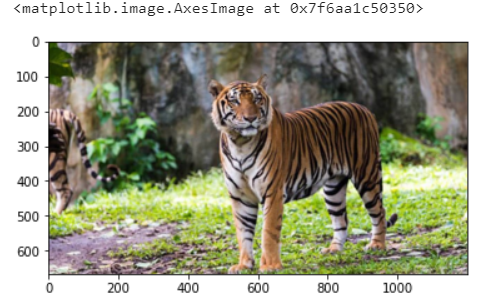
img=cv2.imread('../input/images-for-computer-vision/tiger1.jpg')
The ‘img’ contains the image in the form of a numpy array. Let’s print its type and shape,
print(type(img))
print(img.shape)
The numpy array has a shape of (667, 1200, 3), where,
667 – Image height, 1200 – Image width, 3 – Number of channels,
In this case, there are RGB channels so we have 3. The original image is in the form of RGB but OpenCV reads the image as BGR by default, so we have to convert it back to RGB before displaying it.
Displaying the Image:
# Converting image from BGR to RGB for displaying
img_convert=cv.cvtColor(img, cv.COLOR_BGR2RGB)
plt.imshow(img_convert)
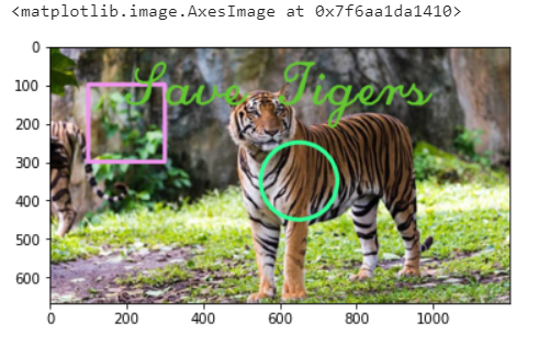
We can draw lines, shapes, and text an image.
# Rectangle
color=(240,150,240) # Color of the rectangle
cv.rectangle(img, (100,100),(300,300),color,thickness=10, lineType=8) ## For filled rectangle, use thickness = -1
## (100,100) are (x,y) coordinates for the top left point of the rectangle and (300, 300) are (x,y) coordinates for the bottom right point
# Circle
color=(150,260,50)
cv.circle(img, (650,350),100, color,thickness=10) ## For filled circle, use thickness = -1
## (250, 250) are (x,y) coordinates for the center of the circle and 100 is the radius
# Text
color=(50,200,100)
font=cv.FONT_HERSHEY_SCRIPT_COMPLEX
cv.putText(img, 'Save Tigers',(200,150), font, 5, color,thickness=5, lineType=20)
# Converting BGR to RGB
img_convert=cv.cvtColor(img, cv.COLOR_BGR2RGB)
plt.imshow(img_convert)
We can also blend two or more images with OpenCV. An image is nothing but numbers, and you can add, subtract, multiply and divide numbers and thus images. One thing to note is that the size of the images should be the same.
# For plotting multiple images at once
def myplot(images,titles):
    fig, axs=plt.subplots(1,len(images),sharey=True)
    fig.set_figwidth(15)
    for img,ax,title in zip(images,axs,titles):
        if img.shape[-1]==3:
            img=cv.cvtColor(img, cv.COLOR_BGR2RGB) # OpenCV reads images as BGR, so converting back them to RGB
        else:
            img=cv.cvtColor(img, cv.COLOR_GRAY2BGR)
        ax.imshow(img)
        ax.set_title(title)
img1 = cv.imread('../input/images-for-computer-vision/tiger1.jpg')
img2 = cv.imread('../input/images-for-computer-vision/horse.jpg')
# Resizing the img1
img1_resize = cv.resize(img1, (img2.shape[1], img2.shape[0]))
# Adding, Subtracting, Multiplying and Dividing Images
img_add = cv.add(img1_resize, img2)
img_subtract = cv.subtract(img1_resize, img2)
img_multiply = cv.multiply(img1_resize, img2)
img_divide = cv.divide(img1_resize, img2)
# Blending Images
img_blend = cv.addWeighted(img1_resize, 0.3, img2, 0.7, 0) ## 30% tiger and 70% horse
myplot([img1_resize, img2], ['Tiger','Horse'])
myplot([img_add, img_subtract, img_multiply, img_divide, img_blend], ['Addition', 'Subtraction', 'Multiplication', 'Division', 'Blending'])
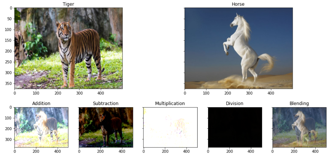
The multiply image is almost white and the division image is black, this is because white means 255 and black means 0. When we multiply two-pixel values of the images, we get a higher number, so its color becomes white or close to white and opposite for the division image.
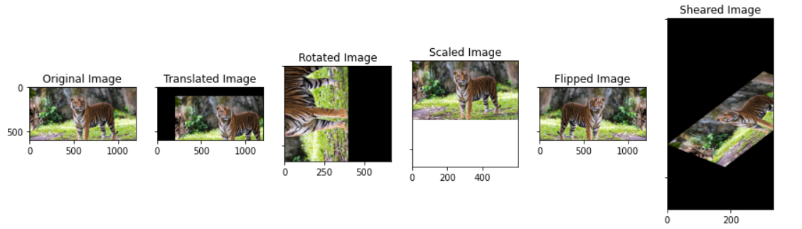
Image transformation includes translating, rotating, scaling, shearing, and flipping an image.
img=cv.imread('../input/images-for-computer-vision/tiger1.jpg')

width, height, _=img.shape


# Translating

M_translate=np.float32([[1,0,200],[0,1,100]]) # 200=> Translation along x-axis and 100=>translation along y-axis

img_translate=cv.warpAffine(img,M_translate,(height,width))


# Rotating

center=(width/2,height/2)

M_rotate=cv.getRotationMatrix2D(center, angle=90, scale=1)

img_rotate=cv.warpAffine(img,M_rotate,(width,height))


# Scaling

scale_percent = 50

width = int(img.shape[1] * scale_percent / 100)

height = int(img.shape[0] * scale_percent / 100)

dim = (width, height)

img_scale = cv.resize(img, dim, interpolation = cv.INTER_AREA)


# Flipping

img_flip=cv.flip(img,1) # 0:Along horizontal axis, 1:Along verticle axis, -1: first along verticle then horizontal


# Shearing

srcTri = np.array( [[0, 0], [img.shape[1] - 1, 0], [0, img.shape[0] - 1]] ).astype(np.float32)

dstTri = np.array( [[0, img.shape[1]*0.33], [img.shape[1]*0.85, img.shape[0]*0.25], [img.shape[1]*0.15, img.shape[0]*0.7]] ).astype(np.float32)

warp_mat = cv.getAffineTransform(srcTri, dstTri)

img_warp = cv.warpAffine(img, warp_mat, (height, width))


myplot([img, img_translate, img_rotate, img_scale, img_flip, img_warp],

       ['Original Image', 'Translated Image', 'Rotated Image', 'Scaled Image', 'Flipped Image', 'Sheared Image'])
Thresholding: In thresholding, the pixel values less than the threshold value become 0 (black), and pixel values greater than the threshold value become 255 (white).
I am taking the threshold to be 150, but you can choose any other number as well.
# For visualising the filters
import plotly.graph_objects as go
from plotly.subplots import make_subplots
def plot_3d(img1, img2, titles):
    fig = make_subplots(rows=1, cols=2,
                    specs=[[{'is_3d': True}, {'is_3d': True}]],
                    subplot_titles=[titles[0], titles[1]],
                    )
    x, y=np.mgrid[0:img1.shape[0], 0:img1.shape[1]]
    fig.add_trace(go.Surface(x=x, y=y, z=img1[:,:,0]), row=1, col=1)
    fig.add_trace(go.Surface(x=x, y=y, z=img2[:,:,0]), row=1, col=2)
    fig.update_traces(contours_z=dict(show=True, usecolormap=True,
                                  highlightcolor="limegreen", project_z=True))
    fig.show()
img=cv.imread('../input/images-for-computer-vision/simple_shapes.png')

# Pixel value less than threshold becomes 0 and more than threshold becomes 255

_,img_threshold=cv.threshold(img,150,255,cv.THRESH_BINARY)

plot_3d(img, img_threshold, ['Original Image', 'Threshold Image=150'])
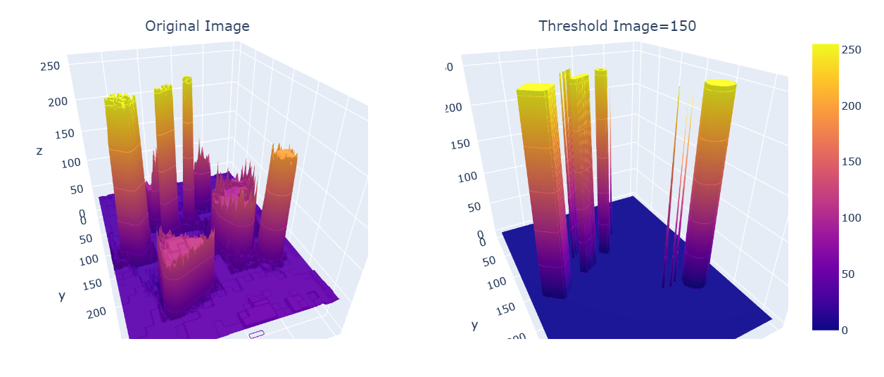
After applying thresholding, the values which are 150 becomes equal to 255
Filtering: Image filtering is changing the appearance of an image by changing the values of the pixels. Each type of filter changes the pixel value based on the corresponding mathematical formula. I am not going into detail math here, but I will show how each filter work by visualizing them in 3D. If you are interested in the math behind the filters, you can check this.
img=cv.imread('../input/images-for-computer-vision/simple_shapes.png')
# Gaussian Filter
ksize=(11,11) # Both should be odd numbers
img_guassian=cv.GaussianBlur(img, ksize,0)
plot_3d(img, img_guassian, ['Original Image','Guassian Image'])
# Median Filter
ksize=11
img_medianblur=cv.medianBlur(img,ksize)
plot_3d(img, img_medianblur, ['Original Image','Median blur'])
# Bilateral Filter
img_bilateralblur=cv.bilateralFilter(img,d=5, sigmaColor=50, sigmaSpace=5)
myplot([img, img_bilateralblur],['Original Image', 'Bilateral blur Image'])
plot_3d(img, img_bilateralblur, ['Original Image','Bilateral blur'])
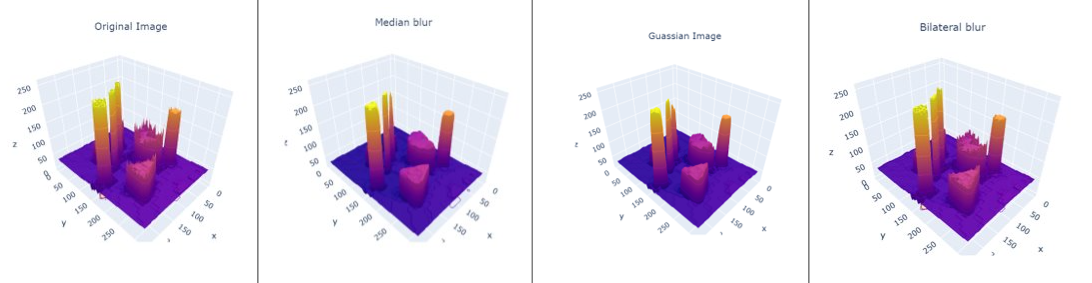
Gaussian Filter: Blurring an image by removing the details and the noise. For more details, you can read this.
Median Filter: Nonlinear process useful in reducing impulsive, or salt-and-pepper noise
Bilateral Filter: Edge-preserving, and noise-reducing smoothing.
In simple words, the filters help to reduce or remove the noise which is a random variation of brightness or color, and this is called smoothing.
Feature detection is a method for making local decisions at every image point by computing abstractions of image information. For example, for an image of a face, the features are eyes, nose, lips, ears, etc. and we try to identify these features.
Let’s first try to identify the edges of an image.
img=cv.imread('../input/images-for-computer-vision/simple_shapes.png')
img_canny1=cv.Canny(img,50, 200)
# Smoothing the img before feeding it to canny
filter_img=cv.GaussianBlur(img, (7,7), 0)
img_canny2=cv.Canny(filter_img,50, 200)
myplot([img, img_canny1, img_canny2],
       ['Original Image', 'Canny Edge Detector(Without Smoothing)', 'Canny Edge Detector(With Smoothing)'])
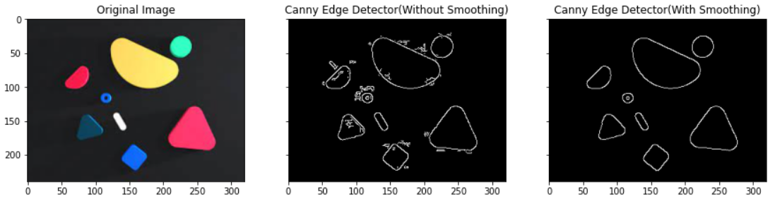
Here we are using the Canny edge detector which is an edge detection operator that uses a multi-stage algorithm to detect a wide range of edges in images. It was developed by John F. Canny in 1986. I am not going in much details of how Canny works, but the key point here is that it is used to extract the edges. To know more about its working, you can check this.
Before detecting an edge using the Canny edge detection method, we smooth the image to remove the noise. As you can see from the image, that after smoothing we get clear edges.
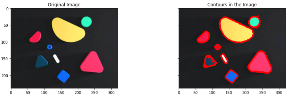
img=cv.imread('../input/images-for-computer-vision/simple_shapes.png')
img_copy=img.copy()
img_gray=cv.cvtColor(img,cv.COLOR_BGR2GRAY)
_,img_binary=cv.threshold(img_gray,50,200,cv.THRESH_BINARY)
#Edroing and Dilating for smooth contours
img_binary_erode=cv.erode(img_binary,(10,10), iterations=5)
img_binary_dilate=cv.dilate(img_binary,(10,10), iterations=5)
contours,hierarchy=cv.findContours(img_binary,cv.RETR_TREE, cv.CHAIN_APPROX_SIMPLE)
cv.drawContours(img, contours,-1,(0,0,255),3) # Draws the contours on the original image just like draw function
myplot([img_copy, img], ['Original Image', 'Contours in the Image'])
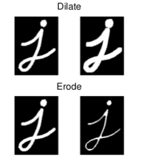
Erode The erosion operation that uses a structuring element for probing and reducing the shapes contained in the image.
Dilation: Adds pixels to the boundaries of objects in an image, simply opposite of erosion
img=cv.imread('../input/images-for-computer-vision/simple_shapes.png',0)
_,threshold=cv.threshold(img,50,255,cv.THRESH_BINARY)
contours,hierarchy=cv.findContours(threshold,cv.RETR_TREE, cv.CHAIN_APPROX_SIMPLE)
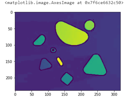
hulls=[cv.convexHull(c) for c in contours]
img_hull=cv.drawContours(img, hulls,-1,(0,0,255),2) #Draws the contours on the original image just like draw function
plt.imshow(img)
We saw how to read and display the image, drawing shapes, text over an image, blending two images, transforming the image like rotating, scaling, translating, etc., filtering the images using Gaussian blur, Median blur, Bilateral blur, and detecting the features using Canny edge detection and finding contours in an image.
I tried to scratch the surface of the computer vision world. This field is evolving each day but the basics will remain the same, so if you try to understand the basic concepts, you will definitely excel in this field.
Lorem ipsum dolor sit amet, consectetur adipiscing elit,