Benchmarking CPU And GPU Performance With Tensorflow

This article was published as a part of the Data Science Blogathon.

Introduction

Hey all✋,

In the past few decades, many revolutions have changed the world we live in, one of them being GPUs. This arrival led us to a new era of computing called AI(Artificial Intelligence) due to the computation power it has to offer.

Nowadays, GPUs have become the new norm. Their impacts can be seen everywhere, from performing scientific calculations to launching rockets and even personal devices such as PCs and Laptops.

Today, we will understand what these GPUs have to offer and how they can increase our productivity. We will also compare the performance of both by training 2 NN’s to recognize digits and pieces of clothing each.

With the goal, set let’s now look at what GPUs are, why to USE them, and their USE CASES.

Understanding GPU

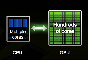
GPUs or Graphical Processing Units are similar to their counterpart but have a lot of cores that allow them for faster computation simultaneously(parallelisim¹). This feature is ideal for performing massive mathematical calculations like calculating image matrices, calculating eigenvalues, determinants, and a lot more.

In a nutshell, one can think of GPU as an extra brain that was always present, but now the power is being harnessed by tech giants like Nvidia & AMD.

Why Use GPU?

There are many reasons to use work on these devices, two most commons are:

Parallelism: One can run code and get a result concisely as all processes are performed in a parallel manner.

Low Latency: Due to the ability to process high intensive calculations, one can expect to get results without delay(i.e., fast computations).

credits

Use Cases of GPU?

Some use cases include:

VDI(Virtual Desktop Infrastructure): One can access the applications from the cloud(CAD), and GPUs can process them in real-time with very low latency.

AI: Due to the ability to process heavy computation, one can teach a machine to mimic humans using neural nets and ml algorithms that primarily work with complex math calculations behind the scenes.

HPC: Most companies can spread their computing among the multiple cluster/nodes/cloud servers and get their job done significantly faster. Thanks to GPU, adding one can dramatically increase the computing time.

I hope this section gave a bit of understanding. Else you can learn more here.

Benchmarking Performance of GPU

Let’s now move on to the 2nd part of the discussion – Comparing Performance For Both Devices Practically. 

For simplicity, I have divided this part into two sections, each covering details of a separate test. Also, former background setting tensorflow_gpu(link in reference) and Jupyter notebook line magic is required.

You can check if TensorFlow is running on GPU by listing all the physical devices as:

tensorflow.config.experimental.list_physical_devices()

or for CUDA friendlies:

tensorflow.test.is_built_with_cuda()

>> True

TEST ONE – Training Digit Classifier

For the 1st test, we will create a digit classifier for the famous cifar10 dataset consisting of  32*32 color images splattered into 50,000 train and 10,000 test images along with ten classes. So lets’ get started.

Here are the steps to do so:

1. Import –  necessary modules and the dataset.

import tensorflow as tf
from tensorflow import keras
import numpy as np
import matplotlib.pyplot as plt

X_train, y_train), (X_test, y_test) = keras.datasets.cifar10.load_data()

2. Perform  Eda – check data and labels shape:

# checking images shape
X_train.shape, X_test.shape

Image By Author

# display single image shape
X_train[0].shape

 

# checking labels
y_train[:5]

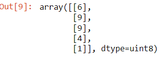
Image By Author

3. Apply Preprocessing: Scaling images(NumPy array) by 255 and One-Hot Encoding labels to represent all categories as 0, except  1 for the actual label in ‘float32.’

# scaling image values between 0-1
X_train_scaled = X_train/255
X_test_scaled = X_test/255

# one hot encoding labels
y_train_encoded = keras.utils.to_categorical(y_train, num_classes = 10, dtype = 'float32')
y_test_encoded = keras.utils.to_categorical(y_test, num_classes = 10, dtype = 'float32')

4. Model Building: A fn to build a neural network with architecture as below with compiling included :

def get_model():
    model = keras.Sequential([
        keras.layers.Flatten(input_shape=(32,32,3)),
        keras.layers.Dense(3000, activation='relu'),
        keras.layers.Dense(1000, activation='relu'),
        keras.layers.Dense(10, activation='sigmoid')    
    ])
    model.compile(optimizer='SGD',
              loss='categorical_crossentropy',
              metrics=['accuracy'])
    return model

Architecture using model.summary() :

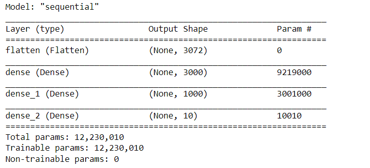
 2 hidden layers having ‘3000 & 1000’ units each followed by softmax layer with ’10 ‘units to output probabilities.- Image By Author

The above codes are self-explanatory. Now let’s train the model and mark the time using the time it magic from jupyter.

5. Training: Train for ten epochs which verbose = 0, meaning no logs.

CPU

%%timeit -n1 -r1
# CPU
with tf.device('/CPU:0'):
    model_cpu = get_model()
    model_cpu.fit(X_train_scaled, y_train_encoded, epochs = 10)

 here -n1 -r1 will ensure the process will run for only one pass, not specifying will perform runs for few no of times and then calculate the average. Also (CPU:0) refers to the first CPU(I have only one).

Image By Author

GPU

%%timeit -n1 -r1
# GPU
with tf.device('/GPU:0'):
    model_gpu = get_model()
    model_gpu.fit(X_train_scaled, y_train_encoded, epochs = 10)

Images By Author

So I think one can understand now why GPUs are preferred. 14~2, really that’s super fast😉.

TEST Two – Training Clothes Classifier

Now let’s confirm our hypothesis by running another test, this time though with fashion mnist dataset, which consists of 28*28 grayscale images split into 60,000 train and 10,000 tests along 10 classes.

Let’s create this one:

# loading dataset
fashion_mnist = keras.datasets.fashion_mnist
(train_images, train_labels), (test_images, test_labels) = fashion_mnist.load_data()

# checking shape

print(train_images.shape)

print(train_labels[0])

>> (60000, 28, 28)
>> 9

# checking images
class_names = ['T-shirt/top', 'Trouser', 'Pullover', 'Dress', 'Coat',
               'Sandal', 'Shirt', 'Sneaker', 'Bag', 'Ankle boot']
plt.imshow(train_images[0])
class_names[train_labels[0]]

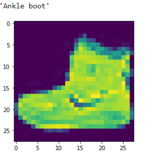
>> Output: Image By Author

# scaling
train_images_scaled = train_images / 255.0
test_images_scaled = test_images / 255.0

Finally, let’s change our model to define how many hidden layers we need for our work and set remote units to be 500. This will allow for a tuning model architecture in case of model overfits.

def get_model(hidden_layers=1):
    # Flatten layer for input
    layers = [keras.layers.Flatten(input_shape=(28, 28))]
    # hideen layers
    for i in range(hidden_layers):
        layers.append(keras.layers.Dense(500, activation='relu'),)
    # output layer    
    layers.append(keras.layers.Dense(10, activation='sigmoid'))
    model = keras.Sequential(layers)
    model.compile(optimizer='adam',
                  loss='sparse_categorical_crossentropy',
                  metrics=['accuracy'])
    return model

If this seems unfamiliar, let me break it down:

In the above code, we store layers as a list and then append those hidden layers as provided in the hidden_layers. Finally, we compile our model with adam as optimizer and sparce_categorical_crossentropy as loss fn. Metric to monitor is again accuracy.

Finally, let’s train our model with 5 hidden layers for 5 epochs:

%%timeit -n1 -r1
with tf.device('/GPU:0'):
    gpu_model = get_model(hidden_layers=5)
    gpu_model.fit(train_images_scaled, train_labels, epochs=5)

Note: Due to certain GPU limitations, epoch runs were needed to be changed from the previous one.

Clearly, this time also GPU’s win the match!😁

Conclusion

we can safely state these are devices essential for computing using neural nets and graphic processings, which require heavy computation.

Also, if you have paid attention to detail, you know how to create a classifier for 2 use cases, a new one to make neural nets, and uses of GPU for TensorFlow.

If you have any concerns feel free to share them in the comments below, or you can directly connect me on LinkedIn, Twitter, or check out my GitHub repo

Lastly, below are the code files and a few additional resources for depth understanding of the topic.

References

Code Files: Github

GPUs: refresher

Inspiration: CodeBasics

Have fun reading🤗

The media shown in this article is not owned by Analytics Vidhya and are used at the Author’s discretion