This article was published as a part of the Data Science Blogathon.
Introduction
In this blog, we will try to solve a famously discussed task of Brain MRI segmentation. Where our task will be to take brain MR images as input and utilize them with deep learning for automatic brain segmentation matured to a level that achieves performance near to a skilled radiologist and then predicts whether a person is identified with a tumor or not.
If there is a tumor detected then we need to provide as much information about the tumor as possible so that this information can be used by doctors to provide better treatment to the patient so and at last we will also try to detect whether a person will survive or not.
In this task, we utilize knowledge of both worlds from deep learning to radiology on this dataset provided by The Cancer Genome Atlas (TCGA) and The Cancer Imaging Archive (TCIA) of 110 different patients and try to generate imaging biomarkers that could provide us with information about the tumor.
This can be classified as a task for supervised learning where we are provided with masks for each image and even our task is to create an image with masks
Lower-grade gliomas are a group of WHO grade II and grade III brain tumors including well-differentiated and anaplastic astrocytomas, oligodendrogliomas, and oligoastrocytomas
Dataset
Dataset for this problem was previously made publicly available by TCGA. Data provided is of image type with *.tif extension and is present in folder with extension ”lgg-mri-segmentation/kaggle_3m/*/*” . This extension here represents all train MR image files whereas for masks extension ends with “_mask”. Apart from these, we are also given a data.csv file that consists of all genome information about each patient.
In the Medical Engineering domain, we generally find less data where a disease is present so generally datasets here are highly imbalanced. But in this case, we find it to be almost balanced.
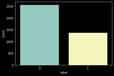
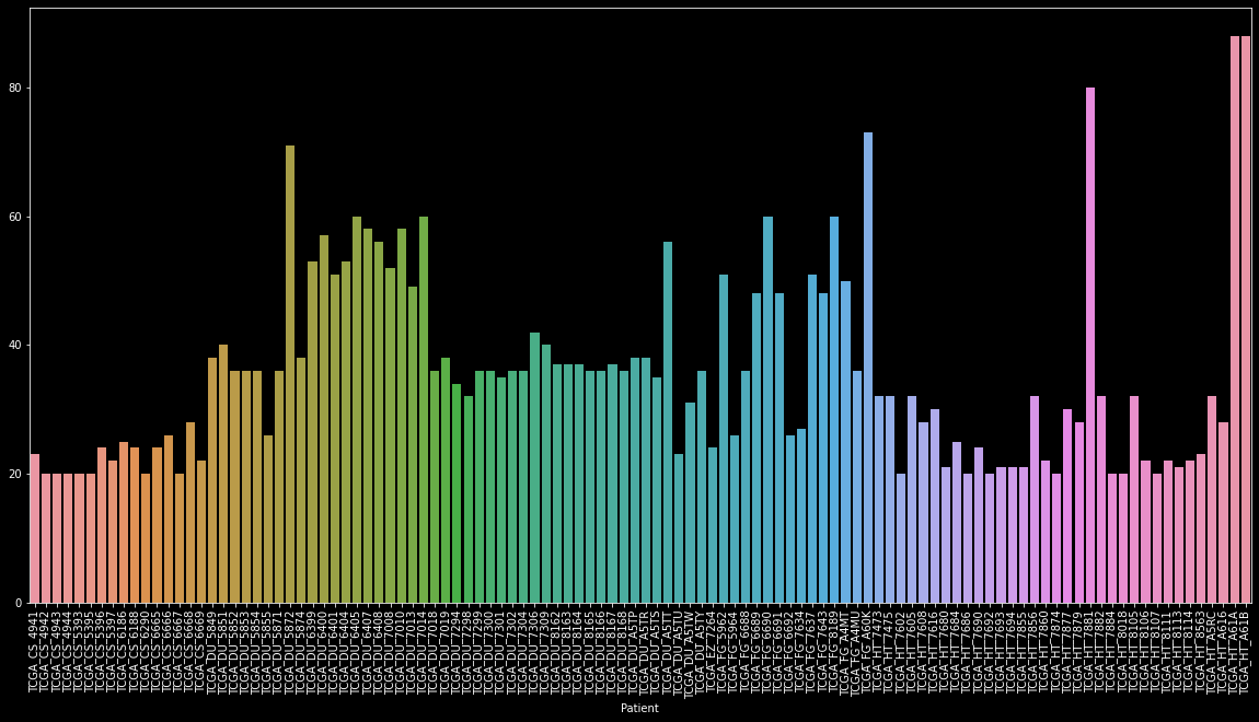
As there are around 3800 images of only 110 patients. This is as we have multiple scans ranging from 20 to 88 per patient.
To make this task simpler this dataset was manually labeled by the creator so we can classify it into supervised learning problems.
this Dataset can be downloaded from here
Method
As our primary objective is to identify more and more features of the tumor so that information can be used by doctors to cure them. some important points that we believe will be beneficial for doctors will be
- Area of tumor
- Coordinates of tumor
- Shape/Spread of the tumor
Gathering all this information we can utilize them to predict almost all visible details about a tumor.
To obtain these data:
- Preprocess data provided and convert it into a model feedable format
- Decide the best suitable metric and losses
- Build a best suitable model architecture
- Tune model performance
- Predict tumor mask
- Analyze the area of mask obtained in which values of pixels are non zero
- Calculate coordinates of the centroid of non-zero pixels
- Obtain std deviation
- Display results
- Use these results to predict the death of a patient
Data preprocessing
Data preprocessing here is the most crucial step as here we do most of our preprocessing and feature engineering stuff. That turns out to be one of the major features of our case study solution.
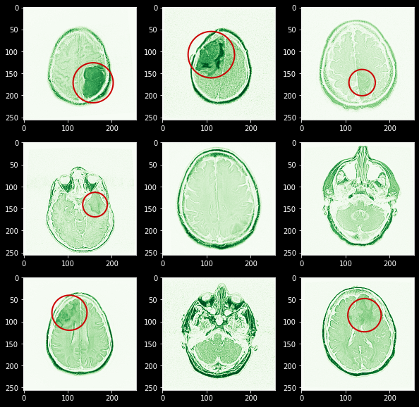
First, let’s have a look at all MR images present for a single patient “TCGA_CS_4941”. Here red circle shows the area where you can identify a tumor
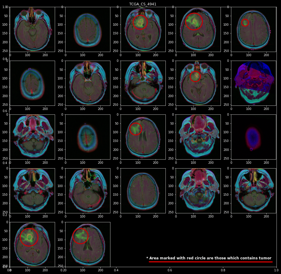
Now as we can see that there are significant numbers of images with tumors. but as we are not trained radiologists or doctors so it turned out that we need to develop some masked images using already test-given masks.
From the above images, we can observe that not all colours in an image are equally useful. it turns out that whenever there is a tumor it gets highlighted with green color thus we can say that whenever there is a high-intensity green colour there may be a tumour, also images here are not too sharp to get the high intensity of each colour therefore we also need an image sharpener, and we don’t need to perform image augmentation as these are image outputs from a standard medical machine. On basis of this observation, we can create a custom data loader class for image preprocessing and data loading combined that should work on this flow chart
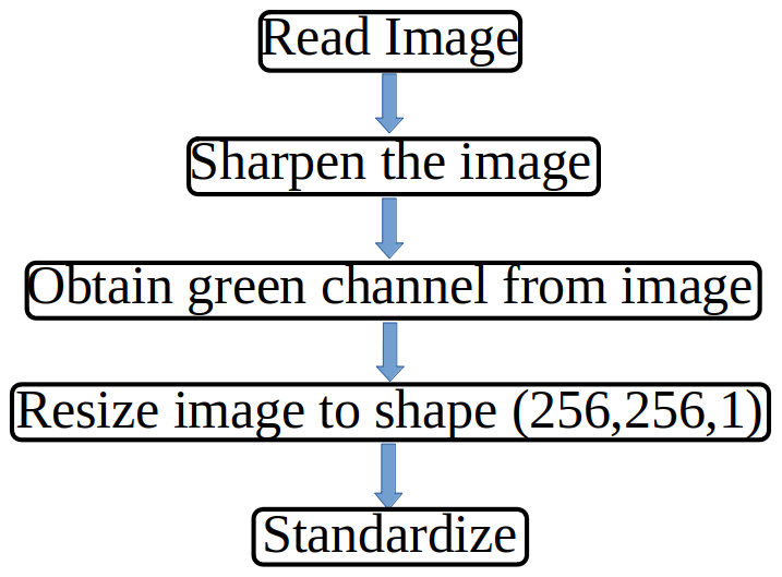
Code for same can be found here
Here in the class dataset we just need to pass a pandas data frame with an image path and mask path along with the patient name and it will return a tuple that contains image and mask.
This tuple is then passed in Dataloader where based on the batch size provided it is being transformed into a model loadable data set.
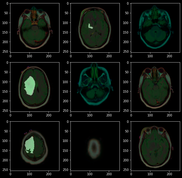
Here you can see I manually marked the area with tumor for red color and also you can observe that it’s fairly easy to visualize this area as these are already marked with high-intensity green color.
Metrics and Losses
As these are tasks for image segmentation. therefore their evaluation metrics are non-trivial to solve. In this, we need a pixel-wise comparison between both the actual mask and the predicted mask.
Therefore there are 2 proposed metrics for semantic segmentation tasks
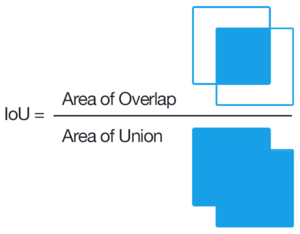
Intersection Over Union(Jaccard Index)
Jaccard Index is one of the most commonly used metrics in semantic segmentation as IoU can be defined as an area of overlap between predicted
segmentation and the ground truth divided by the area of union between
the predicted segmentation and the ground truth. IOU is defined in the range(0-1). Here 0 is defined as no area being overlapped whereas 1 is defined as no noise and the entire defined area being overlapped.
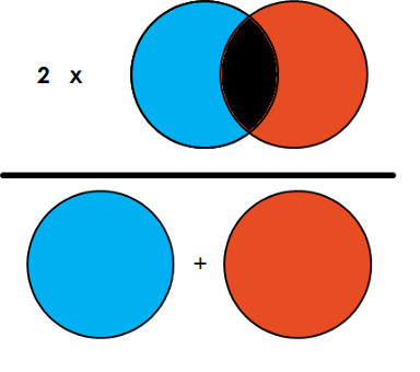
Dice Score(F1 for Semantic segmentation)
Dice score is a useful score that we will use in our case study for evaluation as this metric was first used in paper and till then it is being used to compare your model against others
Dice Coefficient = 2 * the Area of Overlap divided by the total number of pixels in both images.
Losses and metrics can be obtained in Keras using
code:
Model Selection
After going through various models proposed for biomedical image segmentation model proposed we came to the conclusion to use Unet and versions of Unets along with transfer learning. The use of transfer learning will help us reduce training time significantly and obtain better accuracy as using Unet with resnet50 provides an architecture where Resnet 50 acts as a backbone that helps to detect features in images and is pretrained with image net datasets.
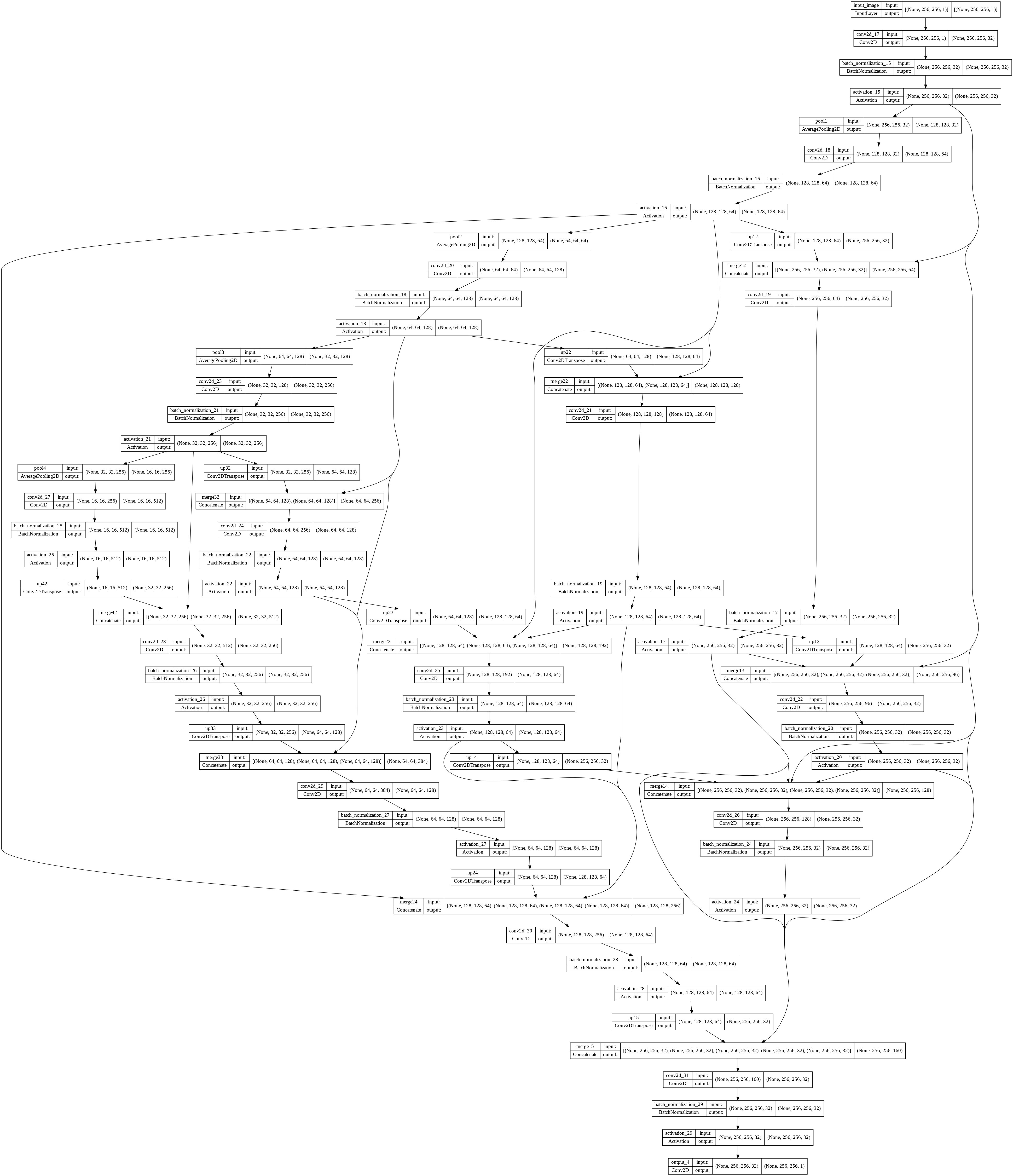
Unet++
This is an Unet architecture with lots of skip connections these skip connections help to obtain particle size features from an image.
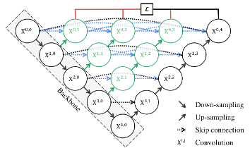
This architecture can be implemented in Keras as
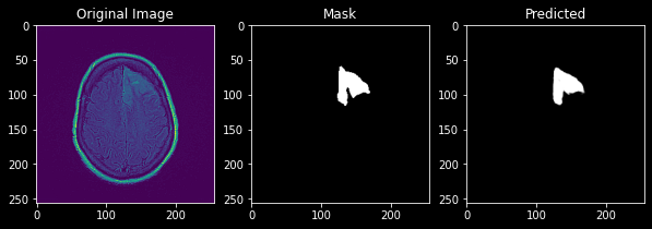
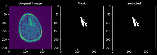
This predicts a mask with a Dice score of 0.9 which is a good score and its predicted image can be viewed as
Unet with Resnet as Backbone
This is an architecture with Resnet encoders as the backbone and the weight of these encoders is frozen.
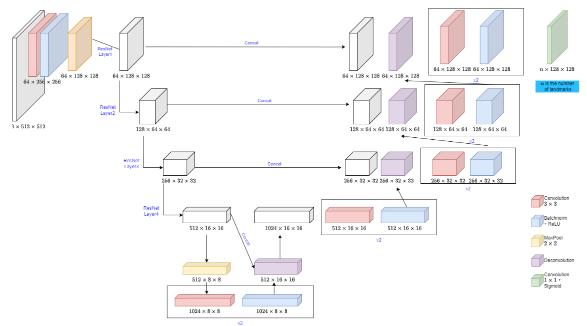
This shows an exceptional Dice score of 0.946
Comparison
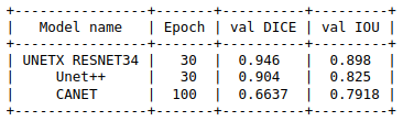
Here we can see the results of each model with DICE and IOU metric and we can also conclude unetxresnet is an architecture that fits our needs.
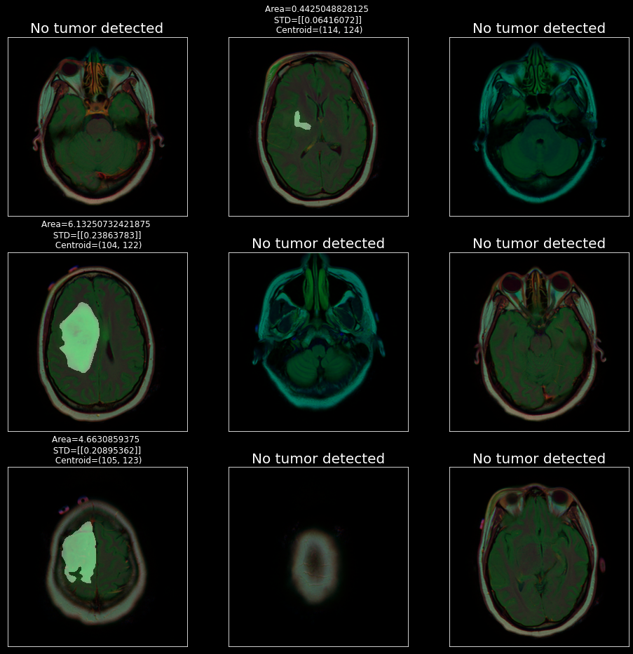
Feature Calculations
Now let’s calculate some important features that will be helpful for doctors to analyze the condition of a patient.
Code:
This function returns area, standard deviation and coordinates
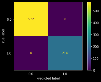
Predict Death
Death01 is a feature present in “lgg-mri-segmentation/kaggle_3m/data.csv” which tells us whether a patient is going to die or not. But there are lots of missing values present in this sheet that needs to be filled up.
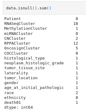
To fill all these unknown values we use an imputer. Here we decide to choose KNNImputer from scikitlearn with n-neighbors=4 and then round it off so as to obtain integer values from the float.
Join both these data frames based on patient ID as key and method as inner join to create another
Now these features can be utilized with provided Data.csv file to predict death01 features as y and it seems that we are able to classify all our points with 100% accuracy
Deployment
Now the major task is to feed this with any image of *.tif format and it should be capable of creating a mask for that image and generating above discussed features. We will not be taking care of Data.csv here. Here we will just generate masks and important features.
For this we will be using stream lit and further code can be downloaded from here.
https://youtu.be/9hwXkstQYZA
Conclusion
This case study discusses various approaches that can be used in process of solving a conventional 2D image segmentation using Keras and Tensorflow. It also discusses what should be the appropriate loss functions and evaluation metrics and how we can just utilize 1 channel from RGB based on EDA to obtain an image with lower dimensions which will help us reduce time and increase performance. We also discussed which features will make a significant impact on doctors and can be extracted from images. On comparing this with other solutions available we found that this approach provides us with the best Dice score ever. Below are some of the key takeaways:
- How Deep-learning and transfer learning can be utilized to solve the task of Biomedical image segmentation
- What should be the best loss function and evaluation metrics for our task
- Generating features from images and utilizing them to predict the death of a patient with 100% accuracy
- Use Streamlit to deploy our model for simpler use
You can find the whole code here: https://github.com/harshnandwana/Brain-mri-segmentation
The media shown in this article is not owned by Analytics Vidhya and is used at the Author’s discretion.


