Introduction
Image segmentation is a task in computer vision that involves dividing a particular image into multiple segments where each segment represents an object or region in the image. This task is important for applications such as object detection, image recognition, and autonomous driving.
TensorFlow is an open-source framework used for building and training machine learning models, in our case image segmentation models. Tensorflow provides the required tools and pre-trained models to perform image segmentation tasks.
Image segmentation has some real-world use cases. They include:
- Object Recognition and Tracking: Image segmentation is used to track and recognize objects such as people, vehicles, and animals in real time. This is mostly used in security systems, surveillance, and autonomous robots.
- Medical Imaging: image segmentation is used to see and segment structures in the body such as organs, tumors, and blood vessels. The data is used for diagnosis, treatment, and research.
- Autonomous Driving: Detecting and classifying objects such as pedestrians and vehicles on the road to avoid accidents and collisions
Learning Objectives
- The goal of this project is to train a model that can create segmentation masks for 59 classes. The first class represents the background of individuals while the remaining 58 classes represent clothing items such as shirts, hair, pants, skin, shoes, glasses, and more.
- In addition to that, is to visualize the masks created by the model from the images and compare them against the correct masks to evaluate the accuracy of the model.
- Furthermore, this aims to provide the user with an understanding of the image segmentation process and how to implement it.
This article was published as a part of the Data Science Blogathon.
Table of Contents
Terminologies
- Deep Learning: is a subset of machine learning that uses neural networks with three or more layers to simulate the behavior of the human brain to learn from data.
- Image Segmentation: The process of dividing an image into segments or regions, each of which represents a separate object or part of the image.
- Mask – a portion of an image that is isolated from the rest of an image.
- Data Augmentation: A way to artificially increase the size of a dataset by applying transformations to existing data.
- Fully Convolutional Neural Network(FCNN) is a neural network that only performs convolution (and subsampling or upsampling) operations. The network comprises three main types of layers: The convolutional layer, the Pooling layer, and Fully-connected layer.
- UNet Architecture: A U-shaped encoder-decoder network architecture comprising four encoder blocks and four decoder blocks joined using a bridge.
- DenseNet121: Architecture consists of four dense blocks and three transition layers. Each dense block has varying numbers of layers featuring two convolutions each to perform the convolution operation.
- Upstack: Also called upsampling or transposed convolutional layers. They are used in the decoder part of the network to increase the spatial resolution of the feature maps.
- Downstack: also called max-pooling layers. They are used in the encoder part of the network to reduce the spatial resolution of the feature maps.
- Skip Connections: are used to connect the corresponding encoder and decoder layers.
Dataset Description
The dataset consists of 1000 images and 1000 corresponding semantic segmentation masks in PNG format. Each image is of size 825 pixels by 550 pixels. The segmentation masks belong to 59 classes, with the first class being the background of individuals and the remaining 58 classes belonging to clothing items for example shirts, hair, pants, skin, shoes, glasses, and more. This dataset is available on Kaggle.
Importing Necessary Libraries and Dependencies
Importing the libraries that are required to perform the tasks in this project.
import os
import cv2
import numpy as np
import tensorflow as tf
from tensorflow import keras
import matplotlib.pyplot as plt
import matplotlib as mpl
from tqdm import tqdm
from sklearn.model_selection import train_test_split
Dataset Preparation
We will begin by creating two separate lists to collect paths for images and mask datasets and then we will iterate over all the files using the os.walk() function. Finally, we will print out the length of both lists.
# a list to collect paths of 1000 images
image_path = []
for root, dirs, files in os.walk('/content/png_images'):
    # iterate over 1000 images
    for file in files:
        # create path
        path = os.path.join(root,file)
        # add path to list
        image_path.append(path)
len(image_path)


# a list to collect paths of 1000 masks
mask_path = []
for root, dirs, files in os.walk('/content/png_masks'):
    #iterate over 1000 masks
    for file in files:
        # obtain the path
        path = os.path.join(root,file)
        # add path to the list
        mask_path.append(path)
len(mask_path)
This prints out a length of 1000 images and 1000 masks respectively.
After sorting out the datasets to get the right image-mask pairs, we will decode the images and masks to store them in separate lists. To do this, we will read each PNG file into memory using a Tensorflow function. They are then decoded into tensors and appended to two separate lists: masks and images.
# create a list to store images
images = []
# iterate over 1000 image paths
for path in tqdm(image_path):
    # read file
    file = tf.io.read_file(path)
    # decode png file into a tensor
    image = tf.image.decode_png(file, channels=3, dtype=tf.uint8)
    # append to the list
    images.append(image)


# create a list to store masks
masks = []
# iterate over 1000 mask paths
for path in tqdm(mask_path):
    # read the file
    file = tf.io.read_file(path)
    # decode png file into a tensor
    mask = tf.image.decode_png(file, channels=1, dtype=tf.uint8)
    # append mask to the list
    masks.append(mask)
Visualizing Dataset Samples
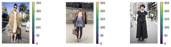
The code below uses matplotlib to create a figure of the images in the range 4 to 6 using a for-loop.
plt.figure(figsize=(25,13))

# Iterate over the images in the range 4-6
for i in range(4,7):
    # Create a subplot for each image
    plt.subplot(4,6,i)
    # Get the i-th image from the list
    img = images[i]
    # Show the image with a colorbar
    plt.imshow(img)
    plt.colorbar()
    # Turn off the axis labels
    plt.axis('off')

# Display the figure
plt.show()
Output:
We again use matplotlib to print out the corresponding masks. We define a normalizer so that the masks have a consistency.
# Define a normalizer that can be applied while visualizing masks to have a consistency
NORM = mpl.colors.Normalize(vmin=0, vmax=58)

# plot masks
plt.figure(figsize=(25,13))
for i in range(4,7):
    plt.subplot(4,6,i)
    img = masks[i]
    plt.imshow(img, cmap='jet', norm=NORM)
    plt.colorbar()
    plt.axis('off')
plt.show()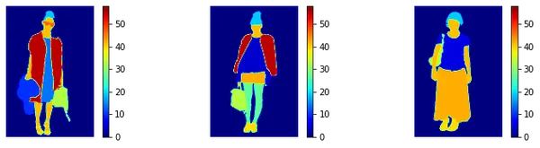
Data Preprocessing
We will start the data preprocessing with two functions to take an image and the corresponding mask from the dataset and resize them to a fixed size of 128 by 128 pixels. The function resize_image will rescale the pixel value and the tf.image.resize will resize the image to the desired size. The mask is resized using the tf.image.resize function without scaling the pixel values. Finally, it converts the data type of the mask tensor to uint8.
We will then use a list comprehension to apply the resizing functions to each image and mask in the original lists of images and masks, respectively. The resulting lists of resized images and masks have the same size as the original lists.
#functions to resize the images and masks
def resize_image(image):
    # scale the image
    image = tf.cast(image, tf.float32)
    image = image/255.0
    # resize image
    image = tf.image.resize(image, (128,128))
    return image

def resize_mask(mask):
    # resize the mask
    mask = tf.image.resize(mask, (128,128))
    mask = tf.cast(mask, tf.uint8)
    return mask


X = [resize_image(i) for i in images]
y = [resize_mask(m) for m in masks]
len(X), len(y)
This prints a length of 1000 in both X and y.
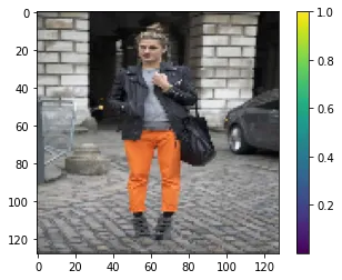
Visualizing a sample of the resized Image and Mask.
#visualizing a resized image and respective mask
# plot an image
plt.imshow(X[36])
plt.colorbar()
plt.show()
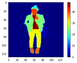
#plot a mask
plt.imshow(y[36], cmap='jet')
plt.colorbar()
plt.show()Output:
Splitting Data into Training and Validation
We will start by splitting the datasets X and y into training and validation sets. The validation data will be 20% of the training data, and the random_state is set to 0 for reproducibility. After that, we will create TensorFlow Dataset objects from the NumPy arrays train_X, val_X, train_y, and val_y using the tensor slices method.
# split data into 80/20 ratio
train_X, val_X,train_y, val_y = train_test_split(X, y, test_size=0.2,
                                                      random_state=0
                                                     )
# develop tf Dataset objects
train_X = tf.data.Dataset.from_tensor_slices(train_X)
val_X = tf.data.Dataset.from_tensor_slices(val_X)

train_y = tf.data.Dataset.from_tensor_slices(train_y)
val_y = tf.data.Dataset.from_tensor_slices(val_y)

# verify the shapes and data types
train_X.element_spec, train_y.element_spec, val_X.element_spec, val_y.element_spec
Data Augmentation
Data augmentation is a way of artificially increasing the training set by creating modified copies of a dataset using existing data. Here are the functions and what they do:
- Brightness: adjusts brightness of the image
- Gamma: adjusts the gamma of the image. The mask is not changed.
- Hue: adjusts the hue of the image. The mask is not transformed.
- Crop: crops the image and the mask and resizes them.
- Flip_hori: function to flip the image and the mask horizontally.
- Flip_vert: function to flip both the image and the mask vertically.
- Rotate: function to rotate both the image and mask by 90 degrees in the clockwise direction.
Each function takes tensors of the image and mask as inputs and returns the resulting image tensor and the original mask tensor. The transformations are designed to be applied identically to both the image and mask tensors so that they stay aligned. This is used to generate new training examples from original data.
# adjust brightness of image
# don't alter in mask
def brightness(img, mask):
    img = tf.image.adjust_brightness(img, 0.1)
    return img, mask

# adjust gamma of image
# don't alter in mask
def gamma(img, mask):
    img = tf.image.adjust_gamma(img, 0.1)
    return img, mask

# adjust hue of image
# don't alter in mask
def hue(img, mask):
    img = tf.image.adjust_hue(img, -0.1)
    return img, mask

def crop(img, mask):
    # crop both image and mask identically
    img = tf.image.central_crop(img, 0.7)
    # resize after cropping
    img = tf.image.resize(img, (128,128))
    mask = tf.image.central_crop(mask, 0.7)
    # resize afer cropping
    mask = tf.image.resize(mask, (128,128))
    # cast to integers as they are class numbers
    mask = tf.cast(mask, tf.uint8)
    return img, mask
# flip both image and mask identically
def flip_hori(img, mask):
    img = tf.image.flip_left_right(img)
    mask = tf.image.flip_left_right(mask)
    return img, mask

# flip both image and mask identically
def flip_vert(img, mask):
    img = tf.image.flip_up_down(img)
    mask = tf.image.flip_up_down(mask)
    return img, mask

# rotate both image and mask identically
def rotate(img, mask):
    img = tf.image.rot90(img)
    mask = tf.image.rot90(mask)
    return img, mask
We will then unzip the images and mask file, apply the augmentation functions, and concatenate the new data to the training set.
# zip images and masks
train = tf.data.Dataset.zip((train_X, train_y))
val = tf.data.Dataset.zip((val_X, val_y))

# perform augmentation on train data only

a = train.map(brightness)
b = train.map(gamma)
c = train.map(hue)
d = train.map(crop)
e = train.map(flip_hori)
f = train.map(flip_vert)
g = train.map(rotate)

# concatenate every new augmented sets
train = train.concatenate(a)
train = train.concatenate(b)
train = train.concatenate(c)
train = train.concatenate(d)
train = train.concatenate(e)
train = train.concatenate(f)
We now have a dataset of the original 800*7=5600 plus the original 800 which is a total of 6400 training examples. After that, the batch size and buffer size are set to get ready for model building.
#setting the batch size
BATCH = 64

AT = tf.data.AUTOTUNE
#buffersize
BUFFER = 1000

STEPS_PER_EPOCH = 800//BATCH
VALIDATION_STEPS = 200//BATCH

train = train.cache().shuffle(BUFFER).batch(BATCH).repeat()
train = train.prefetch(buffer_size=AT)
val = val.batch(BATCH)
Defining and Building the Model
We will use FCNN (Fully Convolutional Neural Networks) which as stated above contains two sections: the encoder(down-stack) and the decoder(up-stack). The encoder is a down-stack of convolutional neural layers that performs the role of extracting features from the input image. A decoder is an up-stack of transposed convolutional neural layers that build the segmented image from the extracted features. In this project, we will use the U-Net architecture.
We wish to use the functional approach of U-Net architecture, but we will have our architecture suitable for our function. The down-stack can be a pre-trained CNN trained for image classification (e.g., MobileNetV2, ResNet, NASNet, Inception, DenseNet, or EfficientNet). It can effectively extract the features. But we have to build our up-stack to match our classes (here, 59), build skip-connections, and train it with our data.
In this case, we will use DenseNet121 from Keras.
# Use pre-trained DenseNet121 without head
base = keras.applications.DenseNet121(input_shape=[128,128,3],
                                      include_top=False,
                                      weights='imagenet')
Next, we define a list of skip-connections for the CNN model. The skip-connections are used to alleviate the vanishing gradient problem in deep neural networks, which can occur when training networks with many layers. The idea is to skip one or more layers and connect earlier layers directly to later layers, allowing gradients to flow more easily during training. They are used in a U-Net architecture to improve the accuracy of semantic segmentation.
#final ReLU activation layer for each feature map size, i.e. 4, 8, 16, 32, and 64, required for skip-connections
skip_names = ['conv1/relu', # size 64*64
             'pool2_relu',  # size 32*32
             'pool3_relu',  # size 16*16
             'pool4_relu',  # size 8*8
             'relu'        # size 4*4
             ]
Building the Downstack
We are building the down-stack, which is used to extract features from the input image and downsample them to reduce the spatial resolution. It uses the DenseNet model, input, output, and weights set not to be updated.
#output of these layers
skip_outputs = [base.get_layer(name).output for name in skip_names]
#Building the downstack with the above layers. We use the pre-trained model as such, without any fine-tuning.
downstack = keras.Model(inputs=base.input,
                       outputs=skip_outputs)
# freeze the downstack layers
downstack.trainable = False
Building the Upstack
An up-stack is used in the decoder part of a U-Net architecture for image segmentation. We will use an up-sampling template for the up-stack pix2pix template which is available open-source in the TensorFlow examples repo.
The up-stack consists of four upsample layers that double the spatial resolution of the feature maps by performing a 2x nearest neighbor upsampling followed by a 3×3 convolutional layer with stride 1. The number of output channels decreases in each successive layer from 512 to 64.
!pip install -q git+https://github.com/tensorflow/examples.git --quiet


from tensorflow_examples.models.pix2pix import pix2pix

# Four upstack layers for upsampling sizes
# 4->8, 8->16, 16->32, 32->64
upstack = [pix2pix.upsample(512,3),
          pix2pix.upsample(256,3),
          pix2pix.upsample(128,3),
          pix2pix.upsample(64,3)]
Building the U-Net model with skip connections by merging the down-stack and up-stack with skip-connections. The code defines the complete U-Net architecture for image segmentation using the down-stack and up-stack layers defined in the prior sections. The down-stack downsamples the images and extracts features, and the up-stack is used to upsample the feature maps to the original input size of the image and concatenate them with the corresponding skip from the down-stack to refine the segmentation output.
Finally, a Conv2DTranspose layer with 59 filters and a kernel size of 3 is applied to the output feature maps to get the final segmentation map.
# define the input layer
inputs = keras.layers.Input(shape=[128,128,3])

# downsample
down = downstack(inputs)
out = down[-1]

# prepare skip-connections
skips = reversed(down[:-1])
# choose the last layer at first 4 --> 8

# upsample with skip-connections
for up, skip in zip(upstack,skips):
    out = up(out)
    out = keras.layers.Concatenate()([out,skip])

# define the final transpose conv layer
# image 128 by 128 with 59 classes
out = keras.layers.Conv2DTranspose(59, 3,
                                  strides=2,
                                  padding='same',
                                  )(out)
# complete unet model
unet = keras.Model(inputs=inputs, outputs=out)
Compiling and Training the Model
A function to compile the model with a learning rate of 0.001 and accuracy as the evaluation metric.
# compiling the model
def Compile_Model():
    unet.compile(loss=keras.losses.SparseCategoricalCrossentropy(from_logits=True),
            optimizer=keras.optimizers.RMSprop(learning_rate=0.001),
            metrics=['accuracy'])
Compile_Model()
Fitting the model on the training set and fine-tuning the model.
#training and fine-tuning
hist_1 = unet.fit(train,
               validation_data=val,
               steps_per_epoch=STEPS_PER_EPOCH,
               validation_steps=VALIDATION_STEPS,
               epochs=20,
               verbose=2)
Making a mask prediction using the model.
# select a validation data batch
img, mask = next(iter(val))
# make prediction
pred = unet.predict(img)
plt.figure(figsize=(20,28))

k = 0
for i in pred:
    # plot the predicted mask
    plt.subplot(4,3,1+k*3)
    i = tf.argmax(i, axis=-1)
    plt.imshow(i,cmap='jet', norm=NORM)
    plt.axis('off')
    plt.title('Prediction')

    # plot the groundtruth mask
    plt.subplot(4,3,2+k*3)
    plt.imshow(mask[k], cmap='jet', norm=NORM)
    plt.axis('off')
    plt.title('Ground Truth')

    # plot the actual image
    plt.subplot(4,3,3+k*3)
    plt.imshow(img[k])
    plt.axis('off')
    plt.title('Actual Image')
    k += 1
    if k == 4: break
plt.suptitle('Predition After 20 Epochs (No Fine-tuning)', color='red', size=20)
plt.show()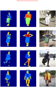
Training the model and fine tuning from the 21st epoch to the 40th epoch.
downstack.trainable = True
# compile again
Compile_Model()
# train from epoch 20 to 40
hist_2 = unet.fit(train,
               validation_data=val,
               steps_per_epoch=STEPS_PER_EPOCH,
               validation_steps=VALIDATION_STEPS,
               epochs=40, initial_epoch = 20,
               verbose = 2
                 )
Making a mask prediction using the model.
# select a validation data batch
img, mask = next(iter(val))
# make prediction
pred = unet.predict(img)
plt.figure(figsize=(20,30))

k = 0
for i in pred:
    # plot the predicted mask
    plt.subplot(4,3,1+k*3)
    i = tf.argmax(i, axis=-1)
    plt.imshow(i,cmap='jet', norm=NORM)
    plt.axis('off')
    plt.title('Prediction')

    # plot the groundtruth mask
    plt.subplot(4,3,2+k*3)
    plt.imshow(mask[k], cmap='jet', norm=NORM)
    plt.axis('off')
    plt.title('Ground Truth')

    # plot the actual image
    plt.subplot(4,3,3+k*3)
    plt.imshow(img[k])
    plt.axis('off')
    plt.title('Actual Image')
    k += 1
    if k == 4: break
plt.suptitle('Predition After 40 Epochs (By Fine-tuning from 21th Epoch)', color='red', size=20)
plt.show()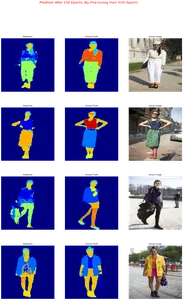
The model has improved greatly.
Performance Curves
We will use the code to visualize the training and validation accuracy of a deep learning model across multiple epochs.
history_1 = hist_1.history
acc=history_1['accuracy']
val_acc = history_1['val_accuracy']

history_2 = hist_2.history
acc.extend(history_2['accuracy'])
val_acc.extend(history_2['val_accuracy'])

plt.plot(acc[:150], '-', label='Training')
plt.plot(val_acc[:150], '--', label='Validation')
plt.plot([50,50],[0.7,1.0], '--g', label='Fine-Tuning')
plt.xlabel('Epochs')
plt.ylabel('Accuracy')
plt.ylim([0.7,1.0])
plt.legend()
plt.show()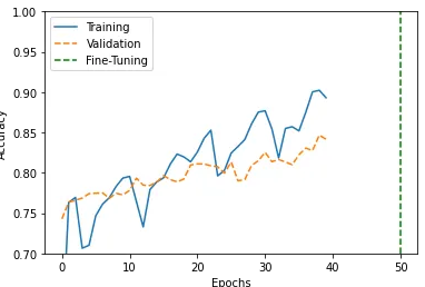
The model would definitely improve with increased epochs and training data.
Conclusion
The project has achieved the objective of training a model that generates masks for the 59 classes of clothing. We were able to compare the generated masks to the corresponding mask in the datasets. We prepared the data, decoded it into tensors, resized, split the dataset, performed data augmentation, and trained the model using the UNet architecture.
- Object segmentation has real-world applications in many fields, including computer vision, medical imaging, robotics, and independent driving.
- The process of object segmentation using TensorFlow includes dataset preparation, data preprocessing, data augmentation, defining the model, splitting data into training and validation sets, and then training and fine-tuning the model to get the desired results.
- Object segmentation can be used to create masks of clothes from random images for use in the fashion industry.
The code is available in my github.
The media shown in this article is not owned by Analytics Vidhya and is used at the Author’s discretion.
I am a Data Scientist and Machine Learning specialist with a passion for uncovering insights and solving complex problems.
I have worked on a wide range of projects, using tools such as python and excel to extract, clean, and analyze data from various sources. I have also developed and trained machine learning models to make predictions and generate insights from data..


