This article was published as a part of the Data Science Blogathon.
Kats model-which is also developed by Facebook Research Team-supports the functionality of multi-variate time-series forecasting in addition to univariate time-series forecasting. Often we need to forecast a time series where we have input variables in addition to ‘time’; this is where the Kats model is valuable.
Kats is a model developed by the Facebook Research team to study time series data. It is an easy-to-use and lightweight framework that helps perform time series analysis. As mentioned earlier, Time series forecasting is an important Data Science component that includes key actions such as characteristics and statistics understanding, anomalies and regressions detection, future trends forecasting, etc.
Time-series forecasting, as the name suggests, is the methodology of learning the patterns in the data, finding if the data shows trend, seasonality, fluctuations, or some variation over time. Various Machine Learning algorithms are currently available for time-series forecasting, such as LSTM, AR, VAR, ARIMA, SARIMA, Facebook Prophet, Kats, etc.
We can have a univariate time series or a multi-variate time series depending on the number of input variables. For multivariate time series forecasting, we use the principle of Vector AutoRegression(VAR).
Vector Autoregression is a model used to find a relationship between multiple variables as they change their values over time. It is a bi-directional model, which means that the variables influence each other, meaning that not only do the predictors influence the target variable, but the target variables also influence the predictors.

Photo by Pablo García Saldaña on Unsplash
This guide will forecast a departmental store’s sales count and visits with five products, namely, A, B, C, D, and E, each with a monthly value of a Sales Count and Visits Count. For simplicity, we will use only one product, A, and predict its Sales Count and Visit Count for the next 3 months.
As a first step, we will initialise the necessary libraries into the Jupyter Notebook.
import pandas as pd
from kats.models.prophet import ProphetModel, ProphetParams
from kats.consts import TimeSeriesData
from kats.models.var import VARModel, VARParams
from sklearn.metrics import r2_score
from sklearn.metrics import mean_squared_error
import math
import numpy as np
import matplotlib.pyplot as plt
Now that the necessary libraries have been initialized, we will be loading our dataset into the notebook next and visualizing it.
df = pd.read_csv("data.csv", index_col=0)
df
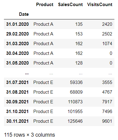
As discussed earlier, for simplicity, we will be forecasting the SalesCount and VisitsCount for only one product out of five in our dataset; we will proceed with only product A.
product = "Product A"
multi_df = df[df["Product"] == product].drop(["Product"], axis=1)
multi_df.head()
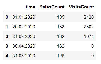
multi_df.reset_index(inplace=True)
multi_df.rename(columns={"Date": "time"},inplace=True)
x=multi_df['time']
y1=multi_df['SalesCount']
y2=multi_df['VisitsCount']
plt.plot(x,y1,y2)
plt.rcParams["figure.figsize"] = (4.8,6.4)
plt.xticks(rotation = 45)
plt.title("Product A Demand over time")
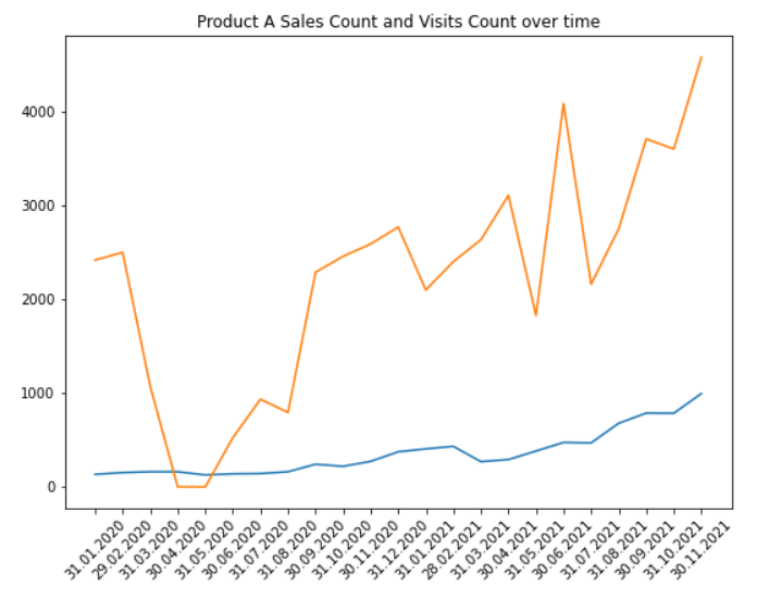
We can see that both the Sales Count and Visits Count are increasing over time.
The next step is to split the dataset into Train and Test datasets. We will be using the Train dataset to train the model and then see how it performs on the unseen data, the Test dataset.
multi_df_train=multi_df[:20]
Wait no more; we will introduce the Kats model into our code and then fit the model onto the Train dataset.
multi_ts = TimeSeriesData(multi_df_train)
params = VARParams()
m = VARModel(multi_ts, params)
m.fit()
Now, we will be forecasting using the Kats model. We just need to run the m.predict function and provide it with the number of steps the model would predict in the future. Kindly note that the step counter starts from the next step of the last timestamp entry of the Train dataset. For example, in our case, the original dataset had monthly date values from 31st January 2020 to 30th November 2021. For the training dataset, we chose the first 19 values with the command multi_df_train=multi_df[:20], so steps=6 would mean that the prediction will be made from the 20th value onwards. Frequency refers to the frequency of the dataset values.
fcst = m.predict(steps=6,freq='M')
Now let us see how the model has produced its forecast.
fcst
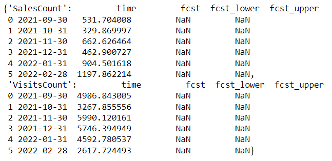
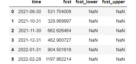
To make the data appear better, let us look at the forecast of the two variables, SalesCount and VisitsCount.
fcst['SalesCount']
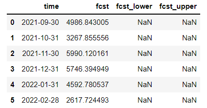
fcst['VisitsCount']
The next step in our guide is to evaluate the performance of the Kats model. We will use Mean Absolute Percentage Error (MAPE) to evaluate our model. SC refers to Sales Count here.
y_pred_sc=sc1['fcst'][:3]
y_true_sc=multi_df['VisitsCount'][20:]
MAPE_SC=mape(y_true_sc,y_pred_sc)
print("n MAPE_SC:n")
print(MAPE_SC*100)
MAPE_SC:
87.35623112447463

y_pred_vc=sc2['fcst'][:3]

y_true_vc=multi_df['VisitsCount'][20:]

MAPE_VC=mape(y_true_vc,y_pred_vc)

print("n MAPE_VC:n")

print(MAPE_VC*100)

MAPE_VC:
24.779222583141625
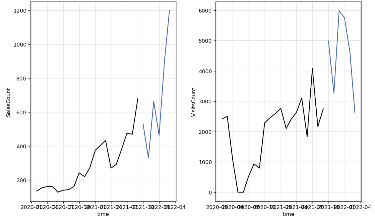
Now, let us plot the actual and predicted curves for both variables.
m.plot()
plt.show()
In this guide, we first learned what the Kats model is, then did a recap on time-series forecasting, particularly multi-variate time-series forecasting. Next, we learned how to use the Kats model for multivariate time-series forecasting using a practical example. We then concluded that Kats is one of the easiest models available in Machine Learning that supports multivariate time-series forecasting. We can list the following takeaways from this article.
The media shown in this article is not owned by Analytics Vidhya and is used at the Author’s discretion.
Lorem ipsum dolor sit amet, consectetur adipiscing elit,


This is a great post! I have been using the Kats model for a while now and it is a great tool for time series forecasting.
Hi! What if we keep the variable "Product"? Can we just fit 1 model considering categorical variable "Product" and get the predictions for each product? Or do we need to fit a model for each product?