This article was published as a part of the Data Science Blogathon.
Introduction
With the rise of meal delivery services, everyone can now enjoy their favorite restaurant food from the comfort of their own home. Giant food aggregators and food shipping companies like Zomato have made it feasible. Zomato is one of India’s most extensively used services for searching restaurants, ordering food online, making table reservations, etc. Bangalore, home to many restaurants and cuisines worldwide, has over 12,000 restaurants doing their business through systems like Zomato. This wide variety is exponentially increasing each day.
The goal of this article and its content is to comprehend the factors that influence the establishment of restaurants in various locations throughout Bangalore; these factors include aggregate consumer score, cuisines offered, type of service provided, and numerous others. With increasingly more eating places, it’s becoming harder for restaurants to run successfully, particularly in a metropolitan metropolis like Bangalore. By studying the Zomato dataset, you can get deeper insights into some of the influencing factors that improve the functioning of a restaurant in Bangalore.
Today, we will investigate a dataset that carries approximate facts about the restaurant chains in Bangalore that also run on Zomato.
Dataset
The dataset used is available to everyone on the Kaggle platform.
Dataset: https://www.kaggle.com/datasets
A description of the dataset:
The dataset has been taken from Kaggle. It contains around 51717 rows and 17 columns of data. The attributes in the dataset are as follows:
- URL: The restaurant’s website URL
- address: Address of the restaurant
- name: Name of the restaurant
- online_orders: It specifies if the restaurant takes online orders or not.
- book_table: Indicates whether or not the restaurant offers table reservations.
- rate: The restaurant’s rating out of 5
- votes: Number of votes received by the restaurant on Zomato
- phone: the restaurant’s phone number
- location: the neighborhood in which the restaurant is located.
- rest_type: specifies the type of restaurant.
- disk_liked: Indicates which dishes were popular among customers in that restaurant.
- Cuisines: Cuisines available at the restaurant
- approx_cost (for two people): Estimated cost of food in that restaurant for two people.
- Reviews_list: Reviews given by users
- menu_item: The restaurant’s menu
- listed_in(type): Specifies the type of service provided by a restaurant
- listed_in(city): The restaurant is on the city’s list.
Objectives
The analysis that we are going to perform shall answer the following questions:
- How many restaurants in Bangalore take online orders?
- What percentage of restaurants offer table booking facilities?
- What was the most common rating received by restaurants?
- Is there any correlation between the approximated cost for two people and the ratings of a restaurant?
- The top five cities in Bangalore with the highest and lowest-rated restaurants.
- Which cuisine do customers like the most?
- What is the average price for two people, based on the type of service?
- Does the restaurant’s rating depend on whether it accepts online orders?
- What are the top 10 highest-rated restaurants?
Implementation
Step 1: Import the libraries
import numpy as np
import pandas as pd
import matplotlib.pyplot as plt
import seaborn as sns
import re
sns.set_style('darkgrid')
Step 2: Load the dataset
You can either download the dataset and then load it into the Jupyter Notebook, or else you can access the dataset by specifying its URL.
Python Code:
import pandas as pd
df = pd.read_csv('zomato.csv')
print(df.head(), end = '\n')
print(df.shape, end = '\n')
print(df.info(), end = '\n')
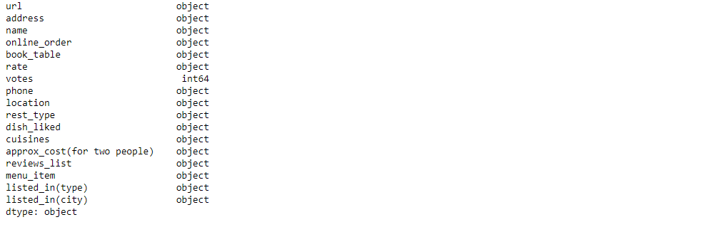
print(df.dtypes, end = '\n')Step 3: Understanding the dataset
df.shape

df.info()
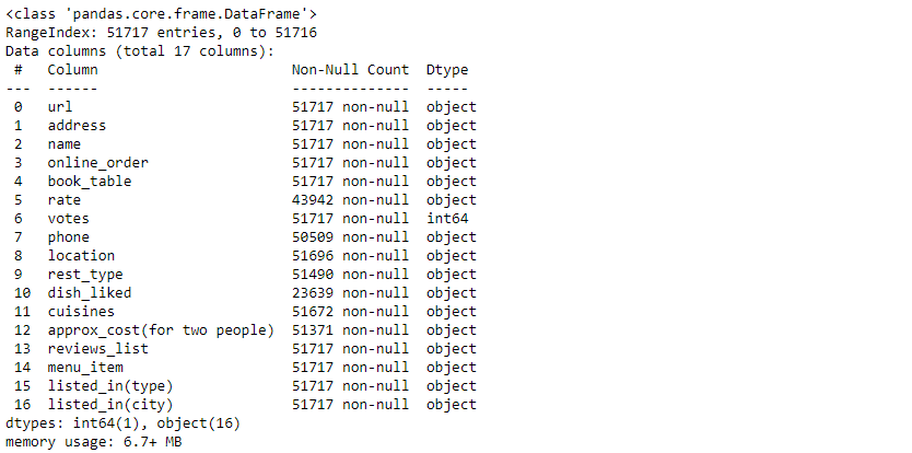
df.dtypes
Step 4: Data Cleaning
(a) Dropping unnecessary columns
Although there are 17 attributes, we will work on only the important ones and remove the remaining columns. Here we only need ‘name’, ‘online order’, ‘book_table’, ‘rate’, ‘votes’, ‘rest_type’, ‘cuisines’, ‘approx_cost(for two people)’, ‘listed_in (type)’, and ‘listed_in(city)’ columns. So, we drop the remaining columns.
df.drop(['url','address','phone','location','dish_liked','reviews_list','menu_item'],axis=1,inplace=True)
(b) Renaming the columns
The columns are then renamed with more descriptive names for easier identification. This is an optional step and can be skipped.
df=df.rename(columns={"name":'Name','rate':'Ratings','votes':'Votes','rest_type':'Rest_Type','cuisines':'Cuisines','approx_cost(for two people)':'Cost','listed_in(type)':'Type','listed_in(city)':'City','online_order':'Takes online orders?','book_table':'Has table booking?'})
df.sample(5)
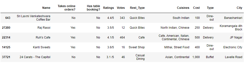
We can see that we now have only 10 columns, and the column names are also replaced.
(c) Dropping duplicate rows
sum(df.duplicated())

Here, we can see that the dataset contains 124 duplicate rows. These rows can sometimes cause a variation in the results and should be taken care of.
df=df.drop_duplicates()
After removing the repeated rows, the shape of the dataframe will be (51593,10).
(d) Cleaning individual rows
(i) First, let’s remove redundant data from the ‘Name’ column. This involves removing punctuation, numbers, special characters, etc., and retaining only alphabets.
def name_clean(text):
    return re.sub(r"[^a-zA-Z0-9 ]", "", text)
df['Name'] = df['Name'].apply(lambda x: name_clean(x))
(ii) Let us now look at the ‘Ratings’ column
df[‘Ratings’].unique()
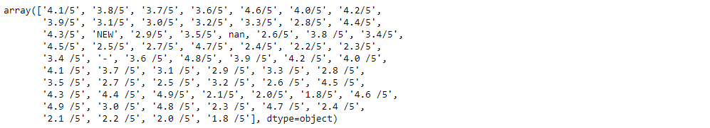
(iii) We can see that we have ‘nan,’ ‘NEW,’ and ‘-‘ values that do not have any ratings, and also, the values are strings containing ‘/5’. Let us remove all insignificant data and convert the ratings into numeric values.
## removing 'nan', 'NEW', '-' values
df["Ratings"]=df["Ratings"].replace("NEW", np.nan)
df['Ratings']=df['Ratings'].replace('NaN',np.nan)
df['Ratings']=df['Ratings'].replace('-',np.nan)
df['Ratings']=df['Ratings'].replace('nan',np.nan)

## function to remove '/5'
def remove_5(value: str):
    if type(value)==str:
        value_new=value.split('/')[0]
        return value_new
    return value
df['Ratings']=df['Ratings'].apply(remove_5)

## converting to float type data

df['Ratings']=df['Ratings'].astype(float)

print(df['Ratings'].dtypes)
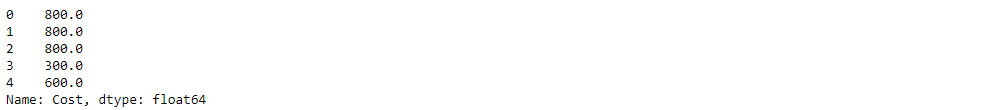
(iv) Noticing the ‘cost’ attribute, we can observe that they are string values containing commas. Below is the code to convert them into numbers.
## function to remove commas and convert the values
## into numbers
def cost(value):
    value = str(value)
    if "," in value:
        value = float(value.replace(",",""))
        return value
    else:
        return float(value)
df['Cost'] = df['Cost'].apply(cost)
print(df['Cost'].head())
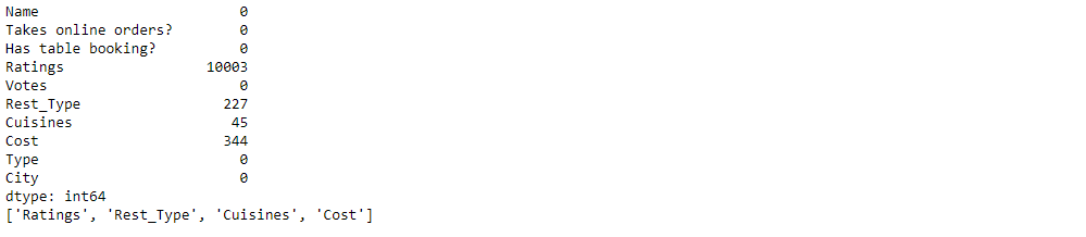
(v) Handling missing data
print(df.isnull().sum())

print([features for features in df.columns if df[features].isnull().sum()>0])
sns.heatmap(df.isnull(),yticklabels=False,cbar=False,cmap='mako')
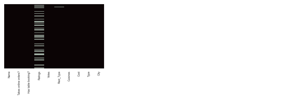
Looking at the above heatmap, we can see a few missing values, particularly in the ‘Ratings’ column. Seeing that now not a good deal of facts is lacking within the other columns, we can drop the corresponding rows.
df=df.dropna()
The data frame reduces to the shape – (41190,10).
Step 5: Exploratory Data Analysis
Now that we have cleaned our data, it is ready for analysis.
- How many restaurants in Bangalore take online orders?
print(df['Takes online orders?'].value_counts())
plt.figure(figsize=(30,10))
df['Takes online orders?'].value_counts().plot(kind='pie',colors=['lightblue','skyblue'],autopct='%1.1f%%', textprops={'fontsize': 15})
plt.title('% of restaurants that take online orders',size=20)
plt.xlabel('',size=15)
plt.ylabel('',size=15)
plt.legend(loc=2, prop={'size': 15})
It is evident from the above graph that in nearly 66% of restaurants, an online ordering facility is available.
- What percentage of restaurants offer table booking facilities?
print(df['Has table booking?'].value_counts())
plt.figure(figsize=(30,10))
df['Has table booking?'].value_counts().plot(kind='pie',colors=['plum','mediumorchid'],autopct='%1.1f%%', textprops={'fontsize': 15})
plt.title('% of restaurants that provide table booking facility',size=20)
plt.xlabel('',size=15)
plt.ylabel('',size=15)
plt.legend(loc=2, prop={'size': 15})
The above pie chart shows that approximately 85% of the restaurants in Bangalore do not have a table booking facility through Zomato.
- What was the most common rating?
ratings=df.groupby(['Ratings']).size().reset_index().rename(columns={0:"Rating_Count"})
plt.figure(figsize=(30,10))
sns.barplot(x='Ratings',y='Rating_Count',data=ratings)
plt.title('Rating vs Rating counts',size=30)
plt.xlabel('Ratings',size=30)
plt.ylabel('Ratings Count',size=30)
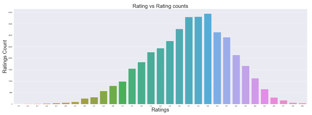
Most of the restaurants in Bangalore received a rating of 3.6 to 4. Very few restaurants have poor ratings, and quite a group of restaurants has excellent ratings of 4.9 or 5.
- Is there any correlation between the two people’s approximated cost and a restaurant’s ratings?
plt.figure(figsize=(30,10))
sns.lmplot(x='Ratings',y='Cost',data=df,height=7)
plt.xlabel('Ratings',size=15)
plt.ylabel('Cost for two people',size=15)
plt.xticks(fontsize=15)
plt.yticks(fontsize=15)
current_values = plt.gca().get_yticks()
plt.gca().set_yticklabels(['{:,.0f}'.format(x) for x in current_values])
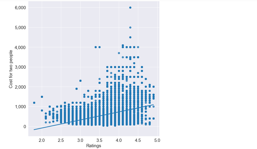
As we can see, restaurants that cost less have better reviews than restaurants that are expensive.
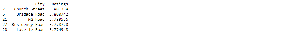
- Top 5 cities in Bangalore that have a maximum number of high and low-rated restaurants.
a=df.groupby('City')['Ratings'].mean().reset_index().sort_values(by='Ratings',ascending=False)
print(a.head())
plt.figure(figsize=(30,10))
plt.barh(a.City,a.Ratings)
plt.xlabel('Ratings',size=15)
plt.ylabel('City',size=15)
plt.xticks(fontsize=15)
plt.yticks(fontsize=15)
plt.title('Average Rating',size=20)
plt.show()
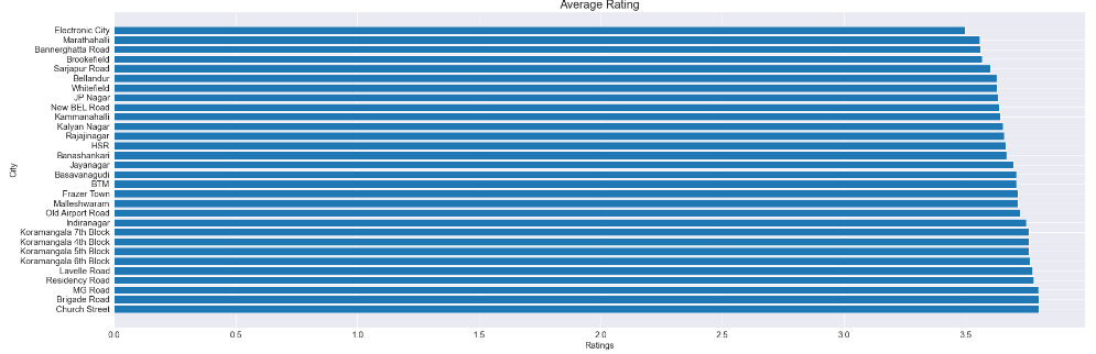
High-rated restaurants are most commonly found in Church Street, Brigade Road, and MG Road, while Electronic City has the lowest number of high-rated restaurants.
- Which cuisine do customers like the most?
Assuming that customers give desirable ratings to their favorite cuisines, the subsequent evaluation is being done:
b=df.groupby('Cuisines')['Ratings'].mean().reset_index().sort_values(by='Ratings',ascending=False)
print(b.head(5))
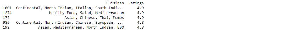
Using searching for the above facts, it may be interpreted that Continental, North Indian, and Italian meals are popular among the restaurant customers in Bangalore.
- What is the average price for two people based on the type of service?
d=df.groupby('Type')['Cost'].mean().reset_index().sort_values(by='Cost')
print(d)
plt.figure(figsize=(30,10))
plt.plot(d['Type'],d['Cost'],'o--r',ms=10)
plt.xlabel('Service type',size=20)
plt.ylabel('Average cost',size=20)
plt.xticks(fontsize=20)
plt.yticks(fontsize=20)
plt.title('Cost based on the type of service provided',size=20)
for i,e in enumerate(d.Cost):
    plt.text(i,e+1,round(e,1),fontsize=15,horizontalalignment='center')
plt.show()
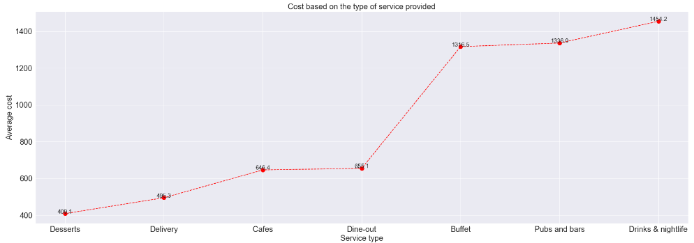
According to the line graph above, while desserts were the least expensive type of food, restaurants that served buffets and drinks cost more than Rs.1300 for two people.
- Does the restaurant’s rating depend on whether it accepts online orders or not?
grp1=df.groupby('Takes online orders?')['Ratings'].mean().reset_index()
plt.figure(figsize=(30,10))
plt.bar(grp1['Takes online orders?'],grp1['Ratings'],alpha=0.5,color='orchid')
plt.xlabel('Takes online orders?',size=20)
plt.ylabel('Average Ratings',size=20)
plt.xticks(fontsize=20)
plt.yticks(fontsize=20)
plt.title('Average rating of restaurants based on whether they take online orders or not',size=20)
plt.show()
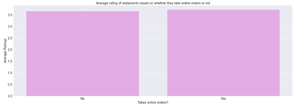
Restaurants receive almost the same average ratings from customers irrespective of whether they take online orders or not. It can be concluded that a restaurant’s success does not largely depend on the facility of taking online orders.
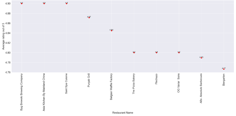
- What are the top 10 highest-rated restaurants?
Often or not, many customers visit a place or choose a place to eat by looking at the restaurant’s ratings. So let us find out the top 10 restaurants that people visit.
grp2=df.groupby('Name')['Ratings'].mean().reset_index().sort_values(by='Ratings',ascending=False)[0:10]
print(grp2)
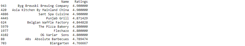
These restaurants happen to receive the highest ratings from customers.
plt.figure(figsize=(30,10))
sns.scatterplot(grp2.Name,grp2.Ratings,s=100,color='red')
for i,e in enumerate(grp2.Ratings):
    plt.text(i,e,round(e,2),fontsize=15,horizontalalignment='center')
plt.xlabel('Restaurant Name',size=20)
plt.ylabel('Average rating out of 5',size=20)
plt.yticks(fontsize=20)
plt.xticks(fontsize=20,rotation=90)
plt.show()
Conclusion
Here, we performed exploratory data analysis on the Zomato Bangalore Restaurants dataset and looked into the most influencing factors that led to a restaurant’s successful running in the city. The code provided here can be easily understood and used to implement EDA on other similar datasets.
Key Takeaways:
- Restaurant ratings are highly influenced by the restaurant’s cuisine, facilities, and pricing.
- The locality where the restaurant is situated also helps in predicting whether the restaurant will run successfully or not.
- Places that sell desserts, beverages, and food delivery services tend to be the most popular among the customers.
The media shown in this article is not owned by Analytics Vidhya and is used at the Author’s discretion.
Data science enthusiast and storyteller. Sharing my learnings and findings from the world of NLP, data science and machine learning through my articles. Let's explore the world of data together! Spreading knowledge, one post at a time.


