Introduction
In recent times, whenever we wish to perform image segmentation in machine learning, the first model we think of is the U-Net. It has been revolutionary in performance improvement compared to previous state-of-the-art methods. U-Net architecture for image segmentation is an encoder-decoder convolutional neural network with extensive medical imaging, autonomous driving, and satellite imaging applications.However, understanding how the U-Net performs segmentation is important, as all novel architectures post-U-Net develop on the same intuition. We will be diving in to understand how the u net segmentation performs image segmentation. To enhance our understanding, we will also apply the U-Net for the task of brain image segmentation.
This article was published as a part of the Data Science Blogathon.
Table of contents
Image Segmentation
Before we get to why U-Net is so popular when it comes to image segmentation tasks, let us understand what image segmentation is. Computer Vision has been one of the many exciting applications of machine intelligence. It has numerous applications in today’s world and makes our lives easier. Two of the most common computer vision tasks are image classification and object detection.
Image classification for two classes involves predicting whether the image belongs to class A or B. The predicted label is assigned to the entire image. Classification is helpful when we want to see what class is in the image.
Object detection, on the other hand, takes this further by predicting the object’s location in our input image. We localize objects within an image by drawing a bounding box around them. Detection is useful for locating and tracking the contents of the image.
Understanding Image Segmentation
One could think of image segmentation as combining classification and localization.
Image segmentation involves partitioning the image into smaller parts called segments. Segmentation involves understanding what is given in an image at a pixel level. It provides fine-grained information about the image as well as the shapes and boundaries of the objects. The output of image segmentation is a mask where each element indicates which class that pixel belongs to. Let’s understand this with an example.
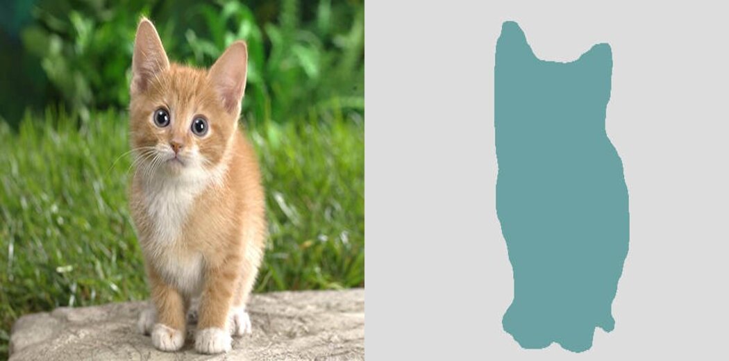
Input and output of image segmentation, respectively
Given above, on the left is our input image of a cat. Our task is to separate the cat from the background. So we have two output classes – cat [1] and background [0]. However, in separating this cat from its background, we need to know the cat’s exact location in the image. We are to find answers to two questions-
- “What” is in the input image?
Ans: Cat and Background - “Where” is that object in the input image?
Ans: The location of the cat in the image
Image segmentation solves the above problem pixel by pixel. We wish to group similar pixels and separate dissimilar pixels. At each pixel, we will perform the classification task of whether that pixel is part of the cat or the background. Thus all the pixels which our model predicts as belonging to the cat will have the label 1, and the remaining pixels will have the label 0. In this process, we would have created a mask of our input image as shown above, and at the end of this pixel-wise classification, we also would have detected the cat’s exact location in our image.
Now that we have understood segmentation let us understand the U-Net model.
Understanding the Development and Advantages of U-Net
Olaf Ronneberger and his team developed u net segmentation in 2015 for their work on biomedical images. It won the ISBI challenge by outperforming the sliding window technique by using fewer images and data augmentation to increase the model performance.
Sliding window architecture performs localization tasks well on any given training dataset. This architecture creates a local patch for each pixel, generating separate class labels for each pixel. However, this architecture has two main drawbacks: firstly, it generates a lot of overall redundancy due to overlapping patches. Secondly, the training procedure was slow, taking a lot of time and resources. These reasons made the architecture not feasible for various tasks. U-Net architecture for image segmentation overcomes these two drawbacks.
U-Net Architecture and its Mechanisms for Image Segmentation
We initially talked about how segmentation consists of classification and localization. Let’s understand how a u net architecture performs these two tasks and why it is so apt for segmentation.
U Net Architecture gets its name from its architecture. The “U” shaped model comprises convolutional layers and two networks. First is the encoder, which is followed by the decoder. With the U-Net, we can solve the above two questions of segmentation: “what” and “where.”

The encoder network is also called the contracting network. This network learns a feature map of the input image and tries to solve our first question- “what” is in the image? It is similar to any classification task we perform with convolutional neural networks except for the fact that in a U-Net, we do not have any fully connected layers in the end, as the output we require now is not the class label but a mask of the same size as our input image.
This encoder network consists of 4 encoder blocks. Each block contains two convolutional layers with a kernel size of 3*3 and valid padding, followed by a Relu activation function. This is inputted to a max pooling layer with a kernel size of 2*2. With the max pooling layer, we have halved the spatial dimensions learned, thereby reducing the computation cost of training the model.
In between the encoder and decoder network, we have the bottleneck layer. This is the bottommost layer, as we can see in the model above. It consists of 2 convolutional layers followed by Relu. The output of the bottleneck is the final feature map representation.
Now, what makes U-Net so good at image segmentation is skip connections and decoder networks. What we have done till now is similar to any CNN. The skip connections and decoder network separates the u net architecture from other CNNs.
Mechanisms of Skip Connections and Decoder Networks
The decoder network is also called the expansive network. Our idea is to up sample our feature maps to the size of our input image. This network takes the feature map from the bottleneck layer and generates a segmentation mask with the help of skip connections. The decoder network tries to solve our second question-“where” is the object in the image? It consists of 4 decoder blocks. Each block starts with a transpose convolution ( indicated as up-conv in the diagram) with a kernel size of 2*2. After concatenating this output with the corresponding skip layer connection from the encoder block, the network utilizes two convolutional layers with a kernel size of 3*3, followed by a Relu activation function.
Skip connections are indicated with a grey arrow in the model architecture. Skip connections help us use the contextual feature information collected in the encoder blocks to generate our segmentation map. The idea is to use our high-resolution features learned from the encoder blocks ( through skip connections ) to help us project our feature map ( output of the bottleneck layer). This helps us answer “where” is our object in the image?
A 1*1 convolution follows the last decoder block with sigmoid activation which gives the output of a segmentation mask containing pixel-wise classification. This way, it could be said that the contracting path passes across information to the expansive path. And thus, we can capture both the feature information and localization with the help of a U-Net.
Let’s take an application of U-Net to understand the model better.
Application in Medical Image Processing
We take the example of brain tumor segmentation. Brain tumor segmentation is a crucial task; early detection increases patients’ survival rates. Manually detecting these tumors is a tedious task. Automating this task using machine learning can help both doctors and patients. Our application tries to predict the brain tumor location using the U-Net.
We use a publicly available dataset. This brain tumor T1-Lighted CE-MRI image dataset consists of 3064 images. There are 1047 coronal images, 990 axial images, and 1027 saggital images. This dataset has a label for each image, identifying the type of tumor. These 3064 images belong to 233 patients. The dataset includes three types of tumors- 708 Meningiomas, 1426 Gliomas, and 930 Pituitary tumors, which are publicly available on: Click Here.
The size of each image is 512X512 pixels. Let’s break down each step of our segmentation project.
Data Loading
We download the dataset from the link given above. The dataset needs to be unzipped and made available. Our dataset is given in matlab format, so we convert this data into numpy arrays each for the images, labels, and masks. We finally display the size of each numpy array.
Our next step is pre-processing this data and visualizing this data. We display the result of each to understand our dataset better.
Next, we normalize the input images. This step is followed by defining our evaluation metrics. We use binary cross-entropy, dice loss, and a custom loss function composed of these two. We also use a 80:10:10 ratio for our train:val:test split and display the size of each.
Now coming to our U-Net model as detailed in our explanation above:
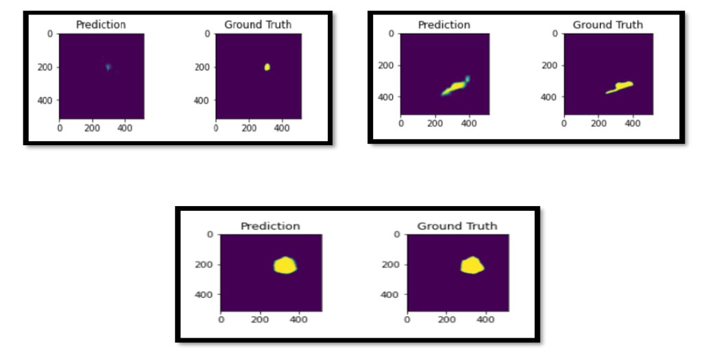
After training this network for 40 epochs, we achieve a dice score of 0.67. Here are a few sample predictions on the test set.
Conclusion
In conclusion, our exploration of image segmentation and U-Net architecture reveals its dual role in classification and localization. By addressing “what” and “where” in segmentation, the encoder captures image content, while the decoder delineates object boundaries. Skip connections facilitate information flow between encoder and decoder, enhancing segmentation accuracy. While we applied U-Net to biomedical tasks, our understanding extends to broader segmentation applications. Future enhancements may involve pre-trained encoder weights and variations on U-Net architecture, yet its fundamental principles endure.
The media shown in this article is not owned by Analytics Vidhya and is used at the Author’s discretion.
Frequently Asked Questions?
Q1. What is the difference between CNN and U-Net?
A. The main difference between CNN and U-Net lies in their architecture and purpose. People commonly use CNN (Convolutional Neural Network) for various tasks like image classification, while researchers specifically designed U-Net for biomedical image segmentation tasks.
Q2. What is U-Net in stable diffusion?
A. U-Net in stable diffusion refers to the application of the U-Net architecture in stable diffusion models, particularly in the context of image denoising and restoration tasks. It leverages U-Net’s capabilities in capturing fine-grained features for effective diffusion-based image processing.
Q3. Why U-Net is good for segmentation?
A. Its unique architecture, which incorporates skip connections between encoder and decoder paths, makes U-Net well-suited for segmentation tasks. These connections help preserve spatial information and enable precise pixel-level segmentation, making U-Net particularly effective for tasks like biomedical image segmentation.
Q4. Who proposed U-Net?
A. Olaf Ronneberger and his team proposed U-Net in 2015 for their work on biomedical image segmentation.


Halfway through reading the article and found it amazing. Excellent!