Introduction

Welcome to an in-depth exploration of ship classification using Convolutional Neural Networks (CNNs) with the Analytics Vidhya hackathon dataset. CNNs are a cornerstone of image-related tasks, known for their ability to learn hierarchical representations of images. In this project, we dive into understanding the power of CNNs to classify ships based on their visual features.

This project aims to demonstrate deep learning application in image categorization and compare CNNs built from scratch and those enhanced through transfer learning. It explores ship classification, from preprocessing to evaluation and comparison.

Learning Objectives

• Apply Convolutional Neural Networks (CNNs) for ship classification.
• Preprocess image data using OpenCV and NumPy.
• Implement CNN models both with and without transfer learning.
• Evaluate model performance using metrics like accuracy and F1-score.
• Compare the results of CNN models with and without transfer learning.

Problem Statement

In this context, the Governmental Maritime and Coastguard Agency seeks to deploy an automated ship detection system leveraging computer vision technology. The objective is to identify and classify ships from images captured by survey boats accurately. With a diverse range of ship types, including cargo ships, tankers, military vessels, carriers, and cruise ships, the challenge lies in developing a robust model capable of distinguishing between these classes effectively.

Dataset Description

The five ship types—Cargo, Tanker, Military, Carrier, and Cruise—are represented in the dataset by a group of photos taken by survey boats. The dataset offers a wide variety of visual data for model construction, with 6252 images for training and 2680 images for testing.

Explanation of OpenCV and CNN

Let us explore about OpenCV and CNN in detail:

OpenCV

With its many features for image processing tasks including object detection, feature extraction, and picture editing, OpenCV is a potent tool. We can improve quality of input photos, identify pertinent features, and preprocess the raw image data by using OpenCV.

Convolutional Neural Networks

CNNs are specifically designed for image-related tasks. CNNs are particularly good at automatically extracting features at various degrees of abstraction from hierarchical representations of images. We can create a model that can recognize unique patterns and traits connected to each type of ship by training a CNN with the labeled ship photos.

Layers in CNNs

CNNs consist of several layers, each serving a specific purpose in processing and extracting features from input images. Let’s break down the components of a CNN:

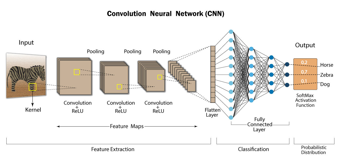
Convolutional Layers

CNNs are mostly composed of convolutional layers. These layers are made up of learnable filters, commonly referred to as kernels, which conduct convolution operations on the input image by sliding over it. The filters use element-wise multiplication and summing operations to extract different features from the input image, including edges, textures, and patterns. Typically, each convolutional layer uses a number of filters to collect various features.

Activation Function

To add non-linearity to the network, an activation function is applied element-by-element to the output feature maps following the convolution operation. Tanh, sigmoid, and ReLU (Rectified Linear Unit) are examples of common activation functions. ReLU’s ease of use and efficiency in solving the vanishing gradient issue make it the most widely utilized activation function in CNNs.

Pooling Layers

Pooling layers downsample the feature maps produced by the convolutional layers to preserve crucial information while reducing their spatial dimensions. The most popular pooling procedure, max pooling, effectively highlights salient features by retaining the maximum value within each pooling region. Pooling the input reduces the network’s computational complexity and enhances its ability to learn robust characteristics, making it more resilient to slight spatial fluctuations.

Fully Connected Layers

Fully connected layers typically perform classification or regression tasks based on the learned features after the convolutional and pooling layers. These layers establish connections between each neuron in a layer and every other layer’s neuron, enabling the network to understand the relationships between features extracted from the input images. In the final phases of network construction, fully connected layers are often used to generate the desired output, such as class probabilities in image classification tasks.

Softmax Layer

Typically, a softmax layer is inserted at the end of the network to transform the class probabilities from the raw output scores in classification tasks. To ensure that the output scores add up to one and can be understood as probabilities, the softmax function normalizes the values for each class. As a result, the network can choose the class with the highest probability to make predictions.

CNNs leverage convolutional layers with learnable filters to extract hierarchical features from input images, followed by activation functions to introduce non-linearity, pooling layers to downsample feature maps, fully connected layers for high-level feature representation, and a softmax layer for classification tasks. This architecture allows CNNs to perform good in various image-related tasks, including image classification, object detection, and segmentation.

Let us now apply the concepts to the dataset from the Analytics Vidhya hackathon.

Implementation of CNN

We’ll execute CNN implementation both with and without transfer learning. To begin, let’s first tackle the implementation without transfer learning.

Here’s the step-by-step implementation:

Step1: Importing Libraries and Dependencies

As we know , the very first step is to install all necessary libraries and dependencies:

import pandas as pd
import numpy as np
import cv2
import seaborn as sns
import tensorflow as tf
import matplotlib.pyplot as plt
from sklearn.model_selection import train_test_split
from tensorflow.keras.models import Sequential
from tensorflow.math import confusion_matrix
from tensorflow.keras.callbacks import ModelCheckpoint
from tensorflow.keras.layers import Conv2D, MaxPooling2D, Flatten, Dense, InputLayer
from glob import glob
from skimage.transform import resize
from keras.utils import to_categorical
from keras.models import Sequential
import keras
from keras.layers import Dense, Conv2D, MaxPool2D , Flatten
from tensorflow.keras import models, layers

Step2: Load the Dataset

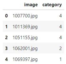
data = pd.read_csv('/kaggle/input/shipdataset/train.csv')

Step3: Data Analysis

Now, let’s conduct some data analysis:

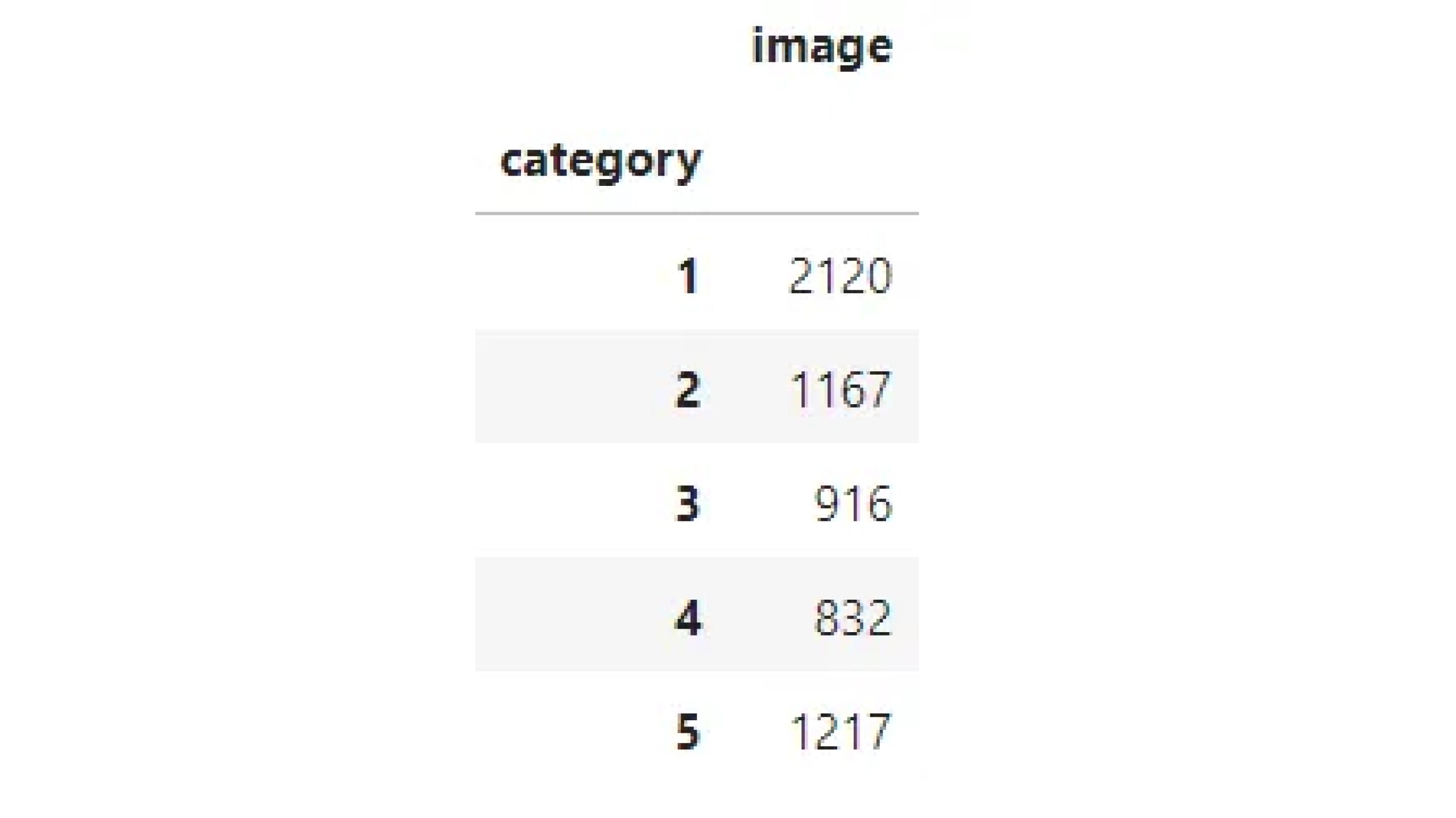
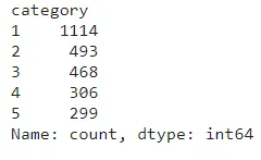
data.groupby('category').count()

This will provide insights into the distribution of categories within the dataset.

Step4: Visualization

Let’s now visualize this:

ship_categories = {1: 'Cargo', 2: 'Military', 3: 'Carrier', 4: 'Cruise', 5: 'Tanker'}
data['category_mapped'] = data['category'].map(ship_categories)
sns.countplot(x='category_mapped', data=data)

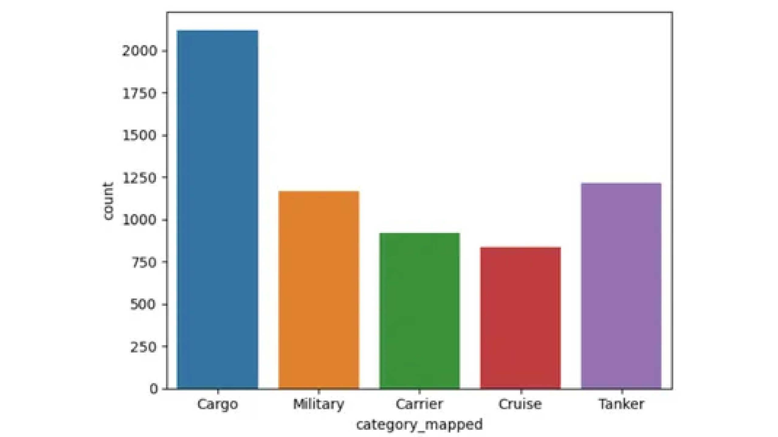
The countplot reveals that the dataset comprises 2120 images categorized as Cargo, 1167 as Military, 916 as Carrier, 832 as Cruise, and 1217 as Tanker.

Step5: Preprocessing the data

Now let’s preprocess the data with the help of code below:

X=[]
import cv2
for img_name in data.image:
    img=cv2.imread('/kaggle/input/shipdataset/images/'+img_name)
    img_resized = cv2.resize(img, (224, 224))
    X.append(img_resized)

X=np.array(X)

This code loads images from a directory, resizes them to 224×224 pixels using OpenCV, and stores the resized images in a NumPy array.

Step6: Plotting

Now let’s plot them after resizing.

nrow = 5
ncol = 4
fig1 = plt.figure(figsize=(15, 15))
fig1.suptitle('After Resizing', size=32)
for i in range(20):
    plt.subplot(nrow, ncol, i + 1)
    plt.imshow(X[i])
    plt.title('class = {x}, Ship = {y}'.format(x=data["category"][i],
     y=ship_categories[data["category"][i]]))
    plt.axis('Off')
    plt.grid(False)
plt.show()

y=data.category.values
y=y-1

This step subtracts 1 from each value in the data.category array, storing the result in the variable y.

The purpose of this operation could be to adjust the category labels. It’s common in machine learning tasks to start indexing from 0 instead of 1, especially when dealing with classification tasks. To align the labels with zero-based indexing, subtracting 1 from the category labels is often done, as required by machine learning algorithms or libraries.

X = X.astype('float32') / 255
y = to_categorical(y)

This code converts pixel values in X to floats between 0 and 1 and one-hot encodes categorical labels in y.

Step7: Data Splitting into Train/Test Dataset

Split the dataset into training and testing sets using the train_test_split function.

X_train, X_test, y_train, y_test = train_test_split(X, y,
 test_size=0.2, random_state=42)

Defining CNN Model: Define a CNN model using TensorFlow’s Sequential API, specifying the convolutional and pooling layers.

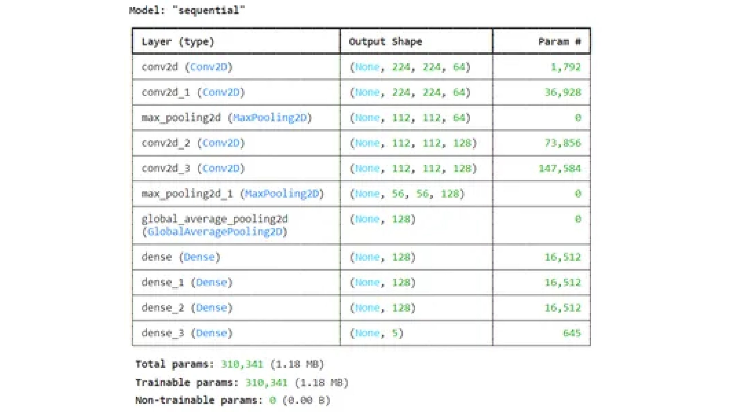
CNN_model = models.Sequential([
    layers.Conv2D(64, (3, 3), activation='relu', padding='same', 
    input_shape=(224, 224, 3)),
    layers.Conv2D(64, (3, 3), padding='same', activation='relu'),
    layers.MaxPooling2D((2, 2)),
    layers.Conv2D(128, (3, 3), padding='same', activation='relu'),
    layers.Conv2D(128, (3, 3), padding='same', activation='relu'), 
    layers.MaxPooling2D((2, 2)),
    layers.GlobalAveragePooling2D(),  
    layers.Dense(128, activation='relu'),
    layers.Dense(128, activation='relu'),
    layers.Dense(128, activation='relu'),
    layers.Dense(5, activation='softmax')  
])
CNN_model.summary()

Step8: Model Training

rain the CNN model on the training data, setting up early stopping and model checkpoint to prevent overfitting and save the best model.

Compile the model with adam optimizer and loss as categorical cross entropy as it’s multiclass classification

from tensorflow.keras.optimizers import Adam
model.compile(optimizer='adam',
                  loss='categorical_crossentropy',
                  metrics=['accuracy',tf.keras.metrics.F1Score()])

Saving the best model on validation loss

from tensorflow.keras.callbacks import EarlyStopping, ModelCheckpoint
early_stop = EarlyStopping(monitor='val_loss', 
patience=3, restore_best_weights=True)
checkpoint = ModelCheckpoint('best_model.keras', 
monitor='val_loss', save_best_only=True, mode='min')

Step9: Fitting the Model

history = model.fit(X_train, y_train, 
                        epochs=20, 
                        batch_size=32, 
                        validation_data=(X_test, y_test), 
                        callbacks=[early_stop, checkpoint])

Step10: Model Evaluation

Now let’s do model evaluation using trained model.

from sklearn.metrics import f1_score
y_pred = model.predict(X_test)

Converting predictions from one-hot encoded format to class labels.

y_pred_labels = np.argmax(y_pred, axis=1)
y_true_labels = np.argmax(y_test, axis=1)

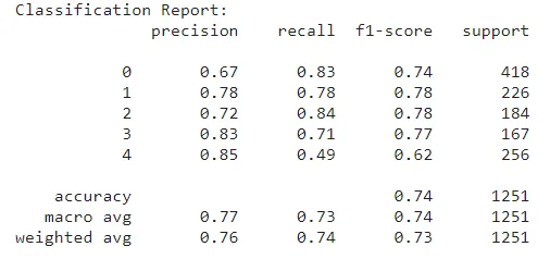
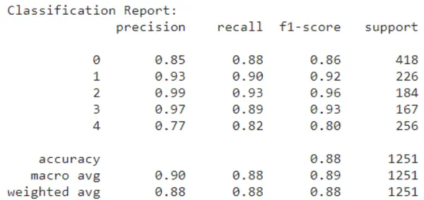
from sklearn.metrics import classification_report
report = classification_report(y_true_labels, y_pred_labels)
print("Classification Report:")
print(report)

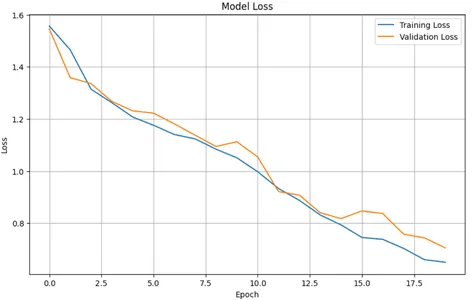
Plotting training & validation loss values

plt.figure(figsize=(10, 6))
plt.plot(history.history['loss'], label='Training Loss')
plt.plot(history.history['val_loss'], label='Validation Loss')
plt.title('Model Loss')
plt.xlabel('Epoch')
plt.ylabel('Loss')
plt.legend()
plt.grid(True)
plt.show()

import matplotlib.pyplot as plt
plt.plot(history.history['accuracy'], label='Training accuracy')
plt.plot(history.history['val_accuracy'], label='Validation accuracy')
plt.title('Training and Validation accuracy')
plt.xlabel('Epoch')
plt.ylabel('Accuracy')
plt.legend()
plt.grid(True)
plt.show()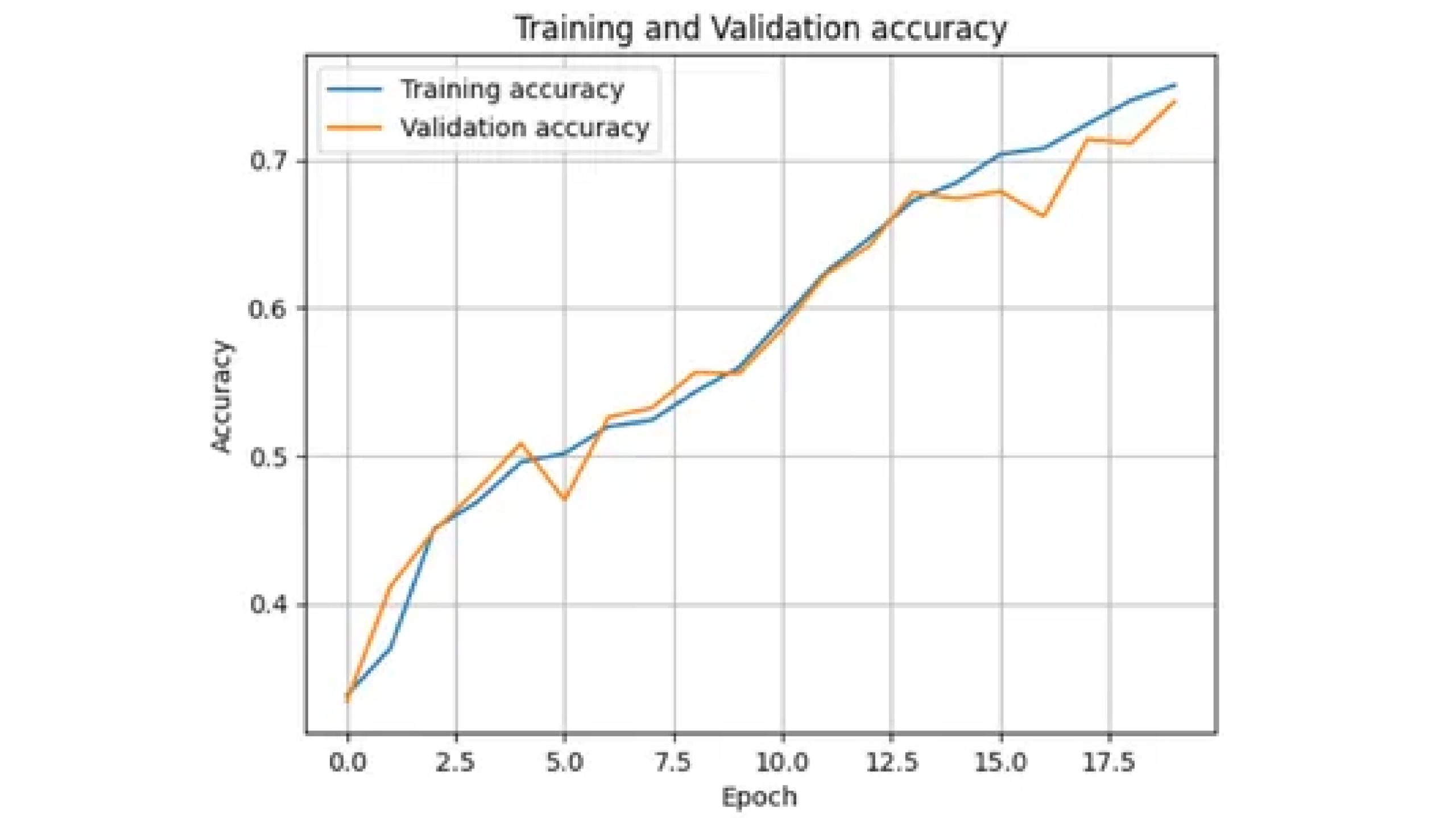

Testing of Data

Preparing and preprocessing the test data similarly to the training data, make predictions using the trained model, and visualize some sample predictions along with their predicted classes.

test=pd.read_csv('/kaggle/input/test-data/test_ApKoW4T.csv')

X_test=[]
import cv2
for img_name in test.image:
    img=cv2.imread('/kaggle/input/shipdataset/images/'+img_name)
    img_resized = cv2.resize(img, (224, 224))
    X_test.append(img_resized)
X_test=np.array(X_test)
X_test = X_test.astype('float32') / 255

Making Prediction

predictions=model.predict(X_test)
predicted_class= np.argmax(predictions,axis=1)
predicted_class=predicted_class+1
csv_=test.copy()
csv_
csv_['category']=predicted_class
csv_.head()

csv_['category'].value_counts()

Save Predictions in CSV

csv_.to_csv('prediction1.csv',index=False)

Plotting the Predicted Test Data

plt.figure(figsize=(8, 8))
for i in range(20):
    plt.subplot(4, 5, i + 1)  
    plt.imshow(X_test[i])  
    plt.title(f'Predicted Class: {ship_categories[predicted_class[i]]}', fontsize=8)  
plt.tight_layout() 
plt.savefig('prediction_plot1.png')
plt.show()

Now let’s use transfer learning to solve this problem for this we will be using resnet.

Understanding Mobilenet

Mobilenet is a type of convolutional neural network (CNN) designed specifically for mobile and embedded devices . It’s known for being efficient and lightweight, making it ideal for situations where processing power and battery life are limited.

Here’s a breakdown of Mobilenet’s key features:

• Efficiency: Mobilenet employs depthwise separable convolutions, which divide data processing into two steps: depthwise convolution using a single filter for each input channel and pointwise convolution using 1×1 filters.
• Lightweight: Mobilenet lowers the amount of parameters needed by the model by minimizing computations. This means that the model will be smaller, which is important for mobile devices with constrained storage.
• Applications: It is useful for various tasks on mobile devices, including image classification, object detection, and facial recognition.

You can read more about MobileNet by clicking here.

We will utilize MobileNet for this task. Everything remains consistent from importing libraries to data splitting(same step as without transfer learning) . Additionally, we need to import the MobileNet library.

from keras.applications import MobileNet
from keras.models import Model
from keras.layers import Dense, GlobalAveragePooling2D
from keras.layers import Dropout, BatchNormalization

Loading Pre-trained Model

Now load the Pre-trained Model as base model

base_model = MobileNet(weights='imagenet', include_top=False)

Freeze all layers in the base model:

for layer in base_model.layers:
    layer.trainable = False

Build Model Using Functional Function 

x = base_model.output
x = GlobalAveragePooling2D()(x)
x = Dense(1024, activation='relu')(x)
x = BatchNormalization()(x)
x = Dropout(0.5)(x)  # Add dropout with a rate of 0.5
predictions = Dense(5, activation='softmax')(x)
 
#Creating the model
model = Model(inputs=base_model.input, outputs=predictions)

Compiling the Model

Compile the model with adam optimizer and loss as categorical cross entropy as it’s multiclass classification

from tensorflow.keras.optimizers import Adam
model.compile(optimizer='adam',
                  loss='categorical_crossentropy',
                  metrics=['accuracy',tf.keras.metrics.F1Score()])

Saving the Best Model on Validation Loss

from tensorflow.keras.callbacks import EarlyStopping, ModelCheckpoint
early_stop = EarlyStopping(monitor='val_loss', patience=2, restore_best_weights=True)
checkpoint = ModelCheckpoint('best_model.keras', monitor='val_loss', 
  save_best_only=True, mode='min')

Fitting the Model

history = model.fit(X_train, y_train, 
                    epochs=20, 
                    batch_size=32, 
                    validation_data=(X_test, y_test),
                    callbacks=[early_stop,checkpoint])

Model Evaluation

Now let’s do model evaluation.

from sklearn.metrics import f1_score

#Making predictions using the trained model
y_pred = model.predict(X_test)

#Converting predictions from one-hot encoded format to class labels
y_pred_labels = np.argmax(y_pred, axis=1)
y_true_labels = np.argmax(y_test, axis=1)

from sklearn.metrics import classification_report
report = classification_report(y_true_labels, y_pred_labels)
print("Classification Report:")
print(report)

Plotting Training and Validation Loss Values

plt.figure(figsize=(10, 6))
plt.plot(history.history['loss'], label='Training Loss')
plt.plot(history.history['val_loss'], label='Validation Loss')
plt.title('Model Loss')
plt.xlabel('Epoch')
plt.ylabel('Loss')
plt.legend()
plt.grid(True)
plt.show()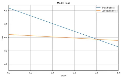

Plotting Accuracy Curve

import matplotlib.pyplot as plt
plt.plot(history.history['accuracy'], label='Training accuracy')
plt.plot(history.history['val_accuracy'], label='Validation accuracy')
plt.title('Training and Validation accuracy')
plt.xlabel('Epoch')
plt.ylabel('Accuracy')
plt.legend()
plt.grid(True)
plt.show()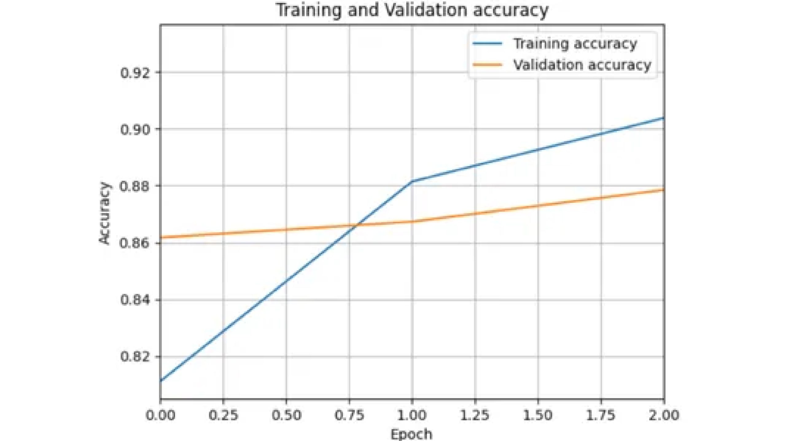

Now do the prediction on test data same as done in without transfer learning

Conclusion

This study explores two approaches to ship classification using Convolutional Neural Networks (CNNs). The first involves building a CNN from scratch without transfer learning techniques, while the second uses transfer learning using MobileNet architecture. Both methods show potential solutions for ship classification, with transfer learning offering better performance with less training data. The choice depends on computational resources, dataset size, and desired performance metrics.

Frequently Asked Questions