Comprehensive Guide on t-SNE Algorithm with Implementation in R & Python

Introduction

Imagine you get a dataset with hundreds of features (variables) and have little understanding of the domain the data belongs to. You are expected to identify hidden patterns and explore and analyze the dataset. And not just that, you have to find out if there is a pattern in the data – is it signal or just noise? In this scenario, employing techniques like t-SNE could prove invaluable in unraveling intricate structures within the dataset.

Does that thought make you uncomfortable? It made my hands sweat when I encountered this situation for the first time. Do you wonder how to explore a multidimensional dataset? It is one of the frequently asked questions by many data scientists. In this article, I will take you through a very powerful way to exactly do this.

What about PCA?

By now, some of you would be screaming “I’ll use PCA for dimensionality reduction and visualization”. Well, you are right! PCA (Principal Component Analysis) is definitely a good choice for dimensionality reduction and visualization for datasets with a large number of features. But, what if you could use something more advanced than PCA? (If you don’t know PCA, I would strongly recommend to read this article first) Feature extraction techniques such as PCA offer a valuable method for reducing the dimensionality of data while preserving most of its important information. Another approach worth considering is KL divergence, which measures the difference between two probability distributions and can be utilized in various machine learning tasks. So, while PCA is widely used and effective, exploring alternatives like feature extraction and KL divergence may provide additional insights and improvements in certain contexts.

What if you could easily search for a pattern in a non-linear style? In this article, I will tell you about a new algorithm called t SNE (2008), which is much more effective than PCA (1933). I will first take you through the basics of the t-SNE algorithm and then explain why t-SNE machine learning is a good fit for dimensionality reduction algorithms.

You will also get hands-on knowledge of using t-SNE in both R and Python.

Read on!

What is t-SNE?

(t-SNE) t-Distributed Stochastic Neighbor Embedding is a non-linear dimensionality reduction algorithm for exploring high-dimensional data. It maps multi-dimensional data to two or more dimensions suitable for human observation. With the help of the t-SNE algorithms, you may have to plot fewer exploratory data analysis plots next time you work with high-dimensional data.

What is Dimensionality Reduction?

To understand how t-SNE works and t-SNE visualization, let’s first understand what dimensionality reduction is.

In simple terms, dimensionality reduction represents multidimensional data (data with multiple features correlating with each other) in two or three dimensions.

Some of you might question why we need dimensional reduction when we can plot the data using scatter plots, histograms & boxplots and make sense of the pattern in data using descriptive statistics. 

Well, even if you can understand the data patterns and present them on simple charts, it is still difficult for anyone without a statistics background to understand them. Also, if you have hundreds of features, you must study thousands of charts before making sense of this data. (Read more about dimensionality reduction here)

With the help of a dimensionality reduction algorithm, you can present the data explicitly.

How does t-SNE Work, and How Can it be Implemented?

t-SNE, or t-Distributed Stochastic Neighbor Embedding, is a method for converting Visualize high-dimensional data into a more manageable form, typically 2D or 3D, facilitating better comprehension. Here’s how it operates:

1. Measure Similarity: Initially, it assesses the similarity between each pair of data points within the high-dimensional space.
2. Map to Lower Dimensions: Subsequently, it endeavors to represent these similarities in a simplified space while preserving the relationships between the points as faithfully as possible.
3. Adjust Positions: It iteratively adjusts the positions of points in the simplified space to align the similarities as closely as feasible.
4. Visualize: Finally, it plots these points in the simplified space, often on a graph, facilitating easier pattern recognition and analysis.

To utilize t SNE, one must prepare the data point, execute the t-SNE algorithm (accessible in libraries like scikit-learn or TensorFlow), and visualize the outcomes. It is a valuable tool for comprehending intricate datasets.

How does t-SNE fit in the dimensionality reduction algorithm space?

Now that you understand what dimensionality reduction is, let’s look at how we can use the t-SNE algorithm to reduce low dimensional points. 

Following are a few dimensionality reduction algorithms that you can check out:

1. PCA (linear)
2. t SNE (non-parametric/ nonlinear)
3. Sammon mapping (nonlinear)
4. Isomap (nonlinear)
5. LLE (nonlinear)
6. CCA (nonlinear)
7. SNE (nonlinear)
8. MVU (nonlinear)
9. Laplacian Eigenmaps (nonlinear)

The good news is that you need to study only two of the abovementioned algorithms to visualize data in lower dimensions – PCA and t SNE effectively.

Limitations of PCA

PCA is a linear algorithm. It cannot interpret complex datasets of polynomial relationships between features. On the other hand, t-SNE machine learning is based on probability distributions with random walks on neighborhood graphs to find the structure of the data.

A major problem with linear dimensionality reduction algorithms is that they concentrate on placing dissimilar data points far apart in a lower-dimension representation. However, to represent high-dimension data on a dimension, non-linear manifold, similar data points must be represented close together, which is not what linear dimensionality reduction algorithms do.

Now, you have a brief understanding of what PCA endeavors to do.

Local approaches seek to map nearby points on the manifold to nearby points in the low-dimensional representation. Global approaches, on the other hand, attempt to preserve geometry at all scales, i.e, mapping nearby points to nearby points and far away points to far away points  

It is important to know that most nonlinear techniques other than t-SNE cannot simultaneously retain the local and global structure of the data.

Algorithmic details of t-SNE (optional read)

This section is for people interested in understanding the algorithm in depth. You can safely skip this section if you do not want to review the math thoroughly.

Let’s understand why you should know about t-SNE and its algorithmic details.  t-SNE is an improvement on the Stochastic Neighbor Embedding (SNE) algorithm.

Algorithm

Step 1

Stochastic Neighbor Embedding (SNE) starts by converting the high-dimensional Euclidean distances between data points into conditional probabilities representing similarities. The similarity of datapoint  to datapoint  is the conditional probability,  ,  would pick as its neighbor if neighbors were picked in proportion to their probability density under a Gaussian centered at . 

For nearby datapoints,  is relatively high, whereas for widely separated datapoints,  will be almost infinitesimal (for reasonable values of the variance of the Gaussian, ). Mathematically, the conditional probability  is given by

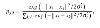
where  is the variance of the Gaussian that is centered on datapoint

If you are not interested in the math, think about it in this way, the algorithm starts by converting the shortest distance (a straight line) between the points into probability of similarity of points. Where, the similarity between points is: the conditional probability that  would pick  as its neighbor if neighbors were picked in proportion to their probability density under a Gaussian distribution centered at .

Step 2

For the low-dimensional counterparts  and  of the high-dimensional datapoints  and   it is possible to compute a similar conditional probability, which we denote by .

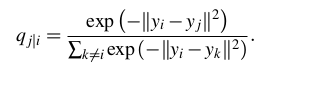
Note that, pi|i and pj|j are set to zero as we only want to model pair wise similarity.

In simple terms step 1 and step2 calculate the conditional probability of similarity between a pair of points in

1. High dimensional space
2. In low dimensional space

 For the sake of simplicity, try to understand this in detail. 

Let us map 3D space to 2D space. What step1 and step2 are calculating the probability of similarity of points in 3D space and calculating the probability of similarity of points in the corresponding 2D space.  

Logically, the conditional probabilities  and must be equal for a perfect representation of the similarity of the datapoints in the different dimensional spaces, i.e the difference between  and  must be zero for the perfect replication of the plot in high and low dimensions.

By this logic SNE attempts to minimize this difference of conditional probability.

Step 3

Now here is the difference between the SNE and t-SNE algorithms. 

To measure the sum of the differences of conditional probability, SNE minimizes the sum of Kullback-Leibler divergence’s overall data points using a gradient descent method. We must know that KL divergences are asymmetric.

In other words, the SNE cost function focuses on retaining the local structure of the data in the map (for reasonable values of the variance of the Gaussian in the high-dimensional space,).

Additionally, it is very difficult (computationally inefficient) to optimize this cost function.

So, t SNE also tries to minimize the sum of the difference in conditional probabilities. But it uses the symmetric SNE cost function version with simple gradients. Also, t-SNE machine learning employs a heavy-tailed distribution in the low-dimensional space to alleviate both the crowding problem (the area of the two-dimensional map that is available to accommodate moderately distant data points will not be nearly large enough compared with the area available to accommodate nearby data points)  and the optimization problems of SNE.

Step 4

If we see the equation to calculate the conditional probability, we have left out the variance from the discussion. The remaining parameter to be selected is the variance of the student’s t-distribution centered over each high-dimensional datapoint . It is not likely that there is a single value of that is optimal for all data points in the data set because the density of the data is expected to vary. In dense regions, a smaller value of  is usually more appropriate than in sparser areas. Any particular value induces a probability distribution,  , over all of the other data points. This distribution has an 

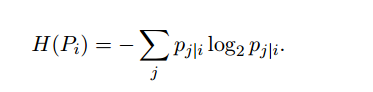
This distribution has an entropy which increases as increases. t-SNE machine learning performs a binary search for the value of  that produces a  with a fixed perplexity that is specified by  the user. The perplexity is defined as

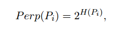
where H() is the Shannon entropy of  measured in bits 

The perplexity can be interpreted as a smooth measure of the effective number of neighbors. The performance of SNE is fairly robust to changes in the perplexity, and typical values are between 5 and 50.

The minimization of the cost function is performed using gradient descent algorithm. And physically, the gradient may be interpreted as the resultant force created by a set of springs between the map point and all other map points  . All springs exert a force along the direction ( – ). The spring between  and repels or attracts the map points depending on whether the distance between the two in the map is too small or too large to represent the similarities between the two high-dimensional datapoints. The force exerted by the spring between and  is proportional to its length, and also proportional to its stiffness, which is the mismatch (pj|i – qj|i + p i| j − q i| j ) between the pairwise similarities of the data points and the map points[1].-

Time and Space Complexity

Now that we have understood the algorithm, it is time to analyze its performance. As you might have observed, the algorithm computes pairwise conditional probabilities and tries to minimize the sum of the difference of the probabilities in higher and lower dimensions. This involves a lot of calculations and computations. So, the algorithm is quite heavy on the system resources.

t-SNE has a quadratic time and space complexity regarding the number of data points. This makes it particularly slow and resource-draining when applied to data sets comprising more than 10,000 observations. 

What Does t-SNE Algorithm Do?

After we have looked into the mathematical description of how the algorithms works, to sum up what we have learned above. Here is a brief explanation of how t-SNE works.  

It’s quite simple: t-sne, a non-linear dimensionality reduction algorithm, finds patterns in the data by identifying observed clusters based on the similarity of data points with multiple features. However, it is not a clustering algorithm but a dimensionality reduction algorithm. It maps the multi-dimensional data to a lower-dimensional space, and the input features are no longer identifiable. Thus, you cannot make any inference based only on the output of t-SNE machine learning. So, essentially, it is mainly a data exploration and visualization technique.

However, t-SNE can be used in classification and clustering by using its output as the input feature for other classification algorithms.

Use Cases

You may ask, what are the use cases of such an algorithm? t-SNE can be used on almost all high-dimensional data sets. However, it is extensively applied in image processing, NLP, genomic data, and speech processing. It has been utilized to improve the analysis of brain and heart scans. Below are a few examples:

Facial Expression Recognition

Much progress has been made on FER, and many algorithms like PCA have been studied for FER. However, FER remains a challenge due to dimension reduction and classification difficulties. t-Stochastic Neighbor Embedding (t SNE) is used to reduce the high-dimensional data into a relatively low-dimensional subspace and then use other algorithms like AdaBoostM2, Random Forests, Logistic Regression, Neural Networks, and others as multi-classifiers for expression classification.

In a recent endeavor focused on facial recognition utilizing the Japanese Female Facial Expression (JAFFE) database, data visualization techniques, specifically t-SNE dimensionality reduction, were employed alongside the AdaBoostM2 algorithm. The experimental findings indicated that the newly proposed algorithm, integrated with t SNE and AdaBoostM2, outperformed traditional approaches like PCA, LDA, LLE, and SNE. This highlights the efficacy of advanced data visualization methods, particularly t-SNE, in enhancing facial expression recognition (FER) systems. Additionally, this project underscores the potential benefits of incorporating such techniques into partner programs to advance facial recognition technology.

The flowchart for implementing such a combination of the data could be as follows:

Preprocessing → normalization → t-SNE→ classification algorithm

                      PCA      LDA    LLE     SNE    t-SNE

SVM               73.5%  74.3%  84.7%  89.6%  90.3%

AdaboostM2   75.4%  75.9%  87.7%  90.6%  94.5%

Identifying Tumor subpopulations (Medical Imaging)

Mass spectrometry imaging (MSI) is a technology that simultaneously provides the spatial distribution for hundreds of biomolecules directly from tissue. Spatially mapped t-distributed stochastic neighbor embedding (t-SNE) is a nonlinear visualization of the data that can better resolve the biomolecular intratumor heterogeneity.

In an unbiased manner, t-SNE machine learning can uncover tumor subpopulations that are statistically linked to patient survival in gastric cancer and metastasis status in primary tumors of breast cancer. Survival analysis performed on each t-SNE cluster will provide significantly useful results.[3]

Text Comparison Using Word2vec

Word vector representations capture many linguistic properties such as gender, tense, plurality, and even semantic concepts like “capital city of”. Using dimensionality reduction, a 2D map can be computed where semantically similar words are close to each other. This combination of techniques can provide a bird’s-eye view of different text sources, including text summaries and their source material. This enables users to explore a text source like a geographical map.[4]

Comparison of t-SNE to Other Dimensionality Reduction Algorithms

While comparing the performance of t-SNE with other algorithms, we will compare t-SNE with other algorithms based on the achieved accuracy rather than the time and resource requirements in relation to accuracy.

t-SNE outputs provide better results than PCA and other linear dimensionality reduction models. This is because a linear method such as classical scaling is not good at modeling curved manifolds. It focuses on preserving the distances between widely separated data points rather than the distances between nearby data points.

The Gaussian kernel employed in the high-dimensional space by t-SNE defines a soft border between the local and global structure of the data. For pairs of data points that are close together relative to the standard deviation of the Gaussian, the importance of modeling their separations is almost independent of the magnitudes of those separations. Moreover, t-SNE machine learning determines the local neighborhood size for each data point separately based on the local density of the data (by forcing each conditional probability distribution to have the same perplexity)[1]. This is because the algorithm defines a soft border between the local and global structure of the data.  And unlike other non-linear dimensionality reduction algorithms, it performs better than any. 

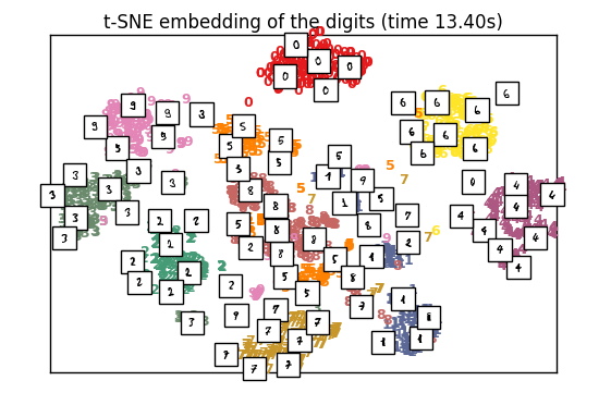
Implementation Using Examples

Let’s implement the t-SNE algorithm on the MNIST handwritten digit database. This is one of the most explored datasets for image processing.

Implementation In R

The “Rtsne” package has an implementation of t SNE in R. The “Rtsne” package can be installed in R using the following command typed in the R console:

install.packages(“Rtsne”)

• Hyperparameter tuning

  

• Code

  MNIST data can be downloaded from the MNIST website and can be converted into a csv file with a

  small amount of code.

  For this example, please download the following preprocessed MNIST data. link

## calling the installed package
train<- read.csv(file.choose()) ## Choose the train.csv file downloaded from the link above  
library(Rtsne)
## Curating the database for analysis with both t-SNE and PCA
Labels<-train$label
train$label<-as.factor(train$label)
## for plotting
colors = rainbow(length(unique(train$label)))
names(colors) = unique(train$label)

## Executing the algorithm on curated data
tsne <- Rtsne(train[,-1], dims = 2, perplexity=30, verbose=TRUE, max_iter = 500)
exeTimeTsne<- system.time(Rtsne(train[,-1], dims = 2, perplexity=30, verbose=TRUE, max_iter = 500))

## Plotting
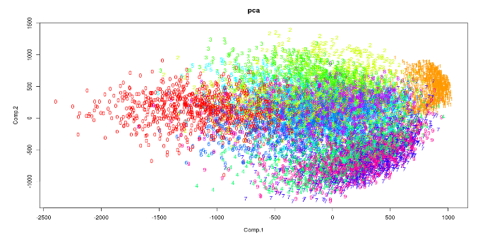
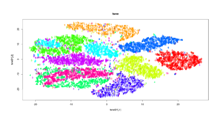
plot(tsne$Y, t='n', main="tsne")
text(tsne$Y, labels=train$label, col=colors[train$label])

• Implementation Time

exeTimeTsne
  user       system  elapsed 
  118.037   0.000  118.006

exectutiontimePCA
   user     system   elapsed 
  11.259   0.012     11.360

As can be seen, t-SNE takes a considerably longer time to execute on the same sample size of data than PCA.  

• Interpreting Results

The plots can be used for exploratory analysis. The output x & y coordinates and cost can be used as features in classification algorithms.

Implementation In Python

An important thing to note is that the “pip install tsne” produces an error. Installing “tsne” package is not recommended. t-SNE algorithm can be accessed from sklearn package.

• Hyperparameter tuning

• Code

The following code is taken from the sklearn examples on the sklearn website.

Python Code:

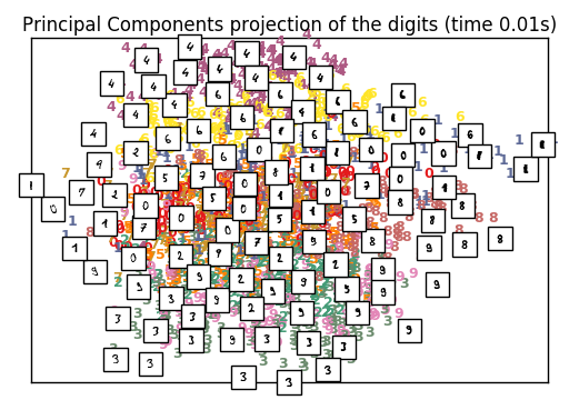
• Implementation Time

Tsne: 13.40 s

PCA: 0.01 s

Where and When to use t-SNE?

How can a Data Scientist use t-SNE?

Well, for the data scientist, the main problem while using t-SNE is the black box-type nature of the algorithm. This impedes the process of providing inferences and insights based on the results. Another problem with the algorithm is that it doesn’t always give a similar output on successive runs.

So then, how could you use the algorithm? The best way to use the algorithm is to use it for exploratory data analysis. It will give you a good sense of patterns hidden inside the data. It can also be used as an input parameter for other classification & clustering algorithms.

How can a Machine Learning Hacker use t-SNE?

Reduce the dataset to 2 or 3 dimensions and stack this with a non-linear stacker. Using a holdout set for stacking/blending. Then, you can boost the t SNE vectors using XGboost to get better results.

How can a Data Science Enthusiasts use t-SNE?

For data science enthusiasts beginning to work with data science, this algorithm presents the best opportunities for research and performance enhancements. A few research papers have attempted to improve the algorithm’s time complexity by utilizing linear functions, but an optimal solution is still required. Research papers on implementing t-SNE for various NLP problems and image processing applications are unexplored territory and have enough scope. Exploring similar data points, utilizing nonlinear dimensionality reduction techniques, and supporting independent authors could significantly contribute to this field’s advancement.

Common Mistakes While Interpreting

Following are a few common fallacies to avoid while interpreting the results of t-SNE:

1. For the algorithm to execute properly, the perplexity should be smaller than the number of points. Also, the suggested perplexity is in the range of (5 to 50)
2. Sometimes, different runs with the same hyperparameters may produce different results.
3. Cluster sizes in any t SNE plot must not be evaluated for standard deviation, dispersion, or any other similar measures. This is because t-SNE machine learning expands denser clusters and contracts sparser clusters to even out cluster sizes, which is one reason for its crisp and clear plots.
4. Distances between clusters may change because global geometry is closely related to optimal perplexity. In a dataset with many clusters with different numbers of elements, one perplexity cannot optimize distances for all clusters.
5. Patterns may also be found in random noise, so multiple runs of the algorithm with different sets of hyperparameters must be checked before deciding if a pattern exists in the data.
6. Different cluster shapes may be observed at different perplexity levels.
7. Topology cannot be analyzed based on a single t-SNE plot; multiple plots must be observed before being assessed.

Conclusion

PCA, a widely used dimensionality reduction method, simplifies data by projecting it onto a lower-dimensional space while preserving the variance. However, it faces challenges when dealing with nonlinear data. On the other hand, t-SNE, which emphasizes local relationships, is adept at visualizing complex structures. While PCA may struggle with nonlinear techniques, t-SNE shines in scenarios where such methods are prevalent. For instance, in facial expression recognition and text comparison using word vectors, t-SNE offers valuable insights. T-SNE machine learning effectively complements PCA and other dimensionality reduction algorithms by highlighting large pairwise distances and redundant features, providing versatile solutions across various domains.

Frequently Asked Questions